Average Return - It’s Not What You Think

📌 Summary & Key Takeaways

• Arithmetic Average Returns Overstate Actual Growth: A stock that drops 50% then gains 100% shows an arithmetic average return of +25% — yet your account balance is completely unchanged. Arithmetic averaging ignores sequence and compounding, consistently distorting investor performance.
• CAGR Measures What Your Balance Actually Earns: Compound Annual Growth Rate (CAGR) calculates the geometric mean — (End Value / Start Value)^(1/Years) - 1 — capturing the exact annualized growth rate required to turn a starting principal into a final balance.
• The Math of Volatility Drag: Expected geometric compound return (\(g\)) is approximated from arithmetic return (\(\mu\)) and annual standard deviation (\(\sigma\)) via \(g \approx \mu - \frac{\sigma^2}{2}\). For an S&P 500 proxy (7.0% arithmetic return, 17.0% volatility), volatility drag deducts ~1.45% annually, pulling simulated 30-year median CAGR down to 5.7% (with outcomes ranging from -6.0% to 18.8% across 10,000 paths).

When I evaluate portfolio performance, one of the most common mistakes I see is using simple arithmetic averaging to measure returns. If you average the last few years of annual percentage gains to determine your expected return, you are calculating a number that overstates your actual wealth accumulation.

In this analysis, I break down the exact mathematical gap between arithmetic averages and geometric Compound Annual Growth Rate (CAGR), and demonstrate why volatility drag systematically reduces realized portfolio growth.

💡 Related Reading: Learn how volatility drag impacts retirement portfolio survival in Safe Withdrawal Rates and explore strategies to reduce drawdown in Defending Your Savings Against Significant Downturns.

A Simple Example: The Volatility Drag Paradox

Consider a straightforward scenario:

I buy a stock at $100, and in Year 1 it drops to $50. My loss is ($50 - $100) / $100 = -50%.

In Year 2, the stock recovers from $50 back to $100. My gain is ($100 - $50) / $50 = +100%.

If I calculate the arithmetic average return, I get: (-50% + 100%) / 2 = +25%.

Yet my starting capital was $100, and my ending capital is $100. I made zero profit.

Claiming a +25% average return when portfolio wealth has not grown at all illustrates why arithmetic averaging is fundamentally flawed for compounding assets.

Investment Returns Compound Geometrically

Portfolio growth depends on compounding. The correct way to calculate net return across multiple periods is by multiplying successive period wealth factors:

($50 / $100) * ($100 / $50) = 0.50 * 2.00 = 1.00

Where r represents the percentage return in a period (expressed as a decimal), each period's return factor (or wealth multiplier) is 1 + r:

• A -50% loss (r = -0.50) gives a return factor of 1 + (-0.50) = 0.50.
• A +100% gain (r = +1.00) gives a return factor of 1 + 1.00 = 2.00.

To get the cumulative wealth multiplier over N periods, I multiply all period factors together: \((1 + r_1) \times (1 + r_2) \times \dots \times (1 + r_N)\).

CAGR measures the constant annual growth rate required to yield the final balance from the initial investment:

$$\text{CAGR} = \left( \frac{\text{End Value}}{\text{Start Value}} \right)^{\frac{1}{\text{Years}}} - 1$$

A Real-World CAGR Example

Suppose I bought a stock index position for $100 in 2010 and sold it for $280 in 2020 (10 years):

$$\text{CAGR} = \left( \frac{280}{100} \right)^{\frac{1}{10}} - 1 = 0.108 = 10.8\%$$

My capital grew at an exact compound rate of 10.8% per year. Reversing the calculation:

$$(1 + 0.108)^{10} = 2.80$$

My initial capital grew by a factor of 2.80 over the 10-year horizon.

The Mathematical Relationship: Calculating Volatility Drag

The gap between arithmetic average return and geometric compound return is governed by portfolio variance. Using a standard Taylor series expansion on logarithmic returns, the expected geometric compound growth rate (\(g\)) is approximated as:

$$\text{Geometric Mean } (g) \approx \text{Arithmetic Mean } (\mu) - \frac{\sigma^2}{2}$$

Where:

• \(\mu\) is the expected arithmetic average annual return.
• \(\sigma\) is the annual standard deviation of returns (volatility).
• \(\frac{\sigma^2}{2}\) is the annual volatility drag.

Let's test this formula against two standard asset allocations:

1. 100% Stock Portfolio (S&P 500 Proxy):

   • \(\mu = 7.0\% = 0.07\)
   • \(\sigma = 17.0\% = 0.17\)
   • \(\text{Volatility Drag} \approx \frac{0.17^2}{2} = \frac{0.0289}{2} = 0.01445 \approx 1.45\%\)
   • Expected Geometric CAGR (\(g\)): \(7.0\% - 1.45\% = \mathbf{5.55\%}\)

2. 60/40 Balanced Portfolio:

   • \(\mu = 5.5\% = 0.055\)
   • \(\sigma = 12.0\% = 0.12\)
   • \(\text{Volatility Drag} \approx \frac{0.12^2}{2} = \frac{0.0144}{2} = 0.0072 = 0.72\%\)
   • Expected Geometric CAGR (\(g\)): \(5.50\% - 0.72\% = \mathbf{4.78\%}\)

Because variance acts as an unavoidable deduction on compounding, a strategy with lower volatility can sometimes achieve higher long-term compounding than a high-volatility strategy with a higher arithmetic average.

Why Monte Carlo Medians Differ from Simple Compounding

When you run a simulation in a Monte Carlo tool (like my Portfolio Accumulation Simulator) with a 7.0% return and 17.0% standard deviation, the engine simulates annual returns drawn from a normal distribution with an arithmetic mean of 7.0%.

Over 30 years, multiplying these randomized annual returns generates the full cone of uncertainty. Because compounding is geometric, the 50th percentile (median) trajectory will compound at approximately 5.55% to 5.70%, not 7.0%.

• Naive Calculation: $300,000 × (1 + 0.07)³⁰ = $2,283,676
• Monte Carlo Geometric Median: $300,000 × (1 + 0.0555)³⁰ ≈ $1,525,000

This is not a bug, an engine fee, or an error. The simulator is showing you the mathematical reality: volatility drag systematically depresses median wealth accumulation.

🔍 Verify the Math in Excel: If you want to verify my simulation math directly against spreadsheet formulas, set the simulator's Standard Deviation to 0.0%. Eliminating volatility removes all random variance, causing the simulation to collapse into pure deterministic compounding (\(P_0 \times (1 + r)^t\)) that matches spreadsheet formulas to the exact penny.

Quantification of Volatility Drag: 10,000-Path Monte Carlo Simulation

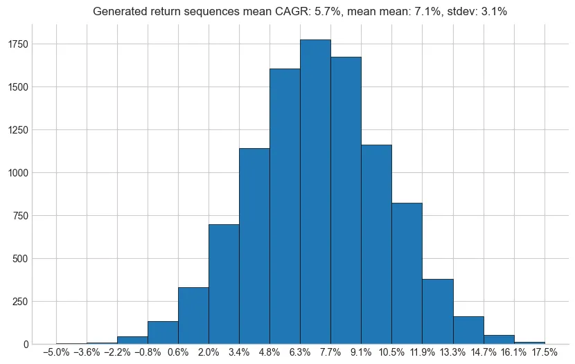
To quantify how annual return variance depresses realized CAGR below arithmetic return expectations, I simulated 10,000 independent 30-year market sequences. Each sequence drew annual returns from a normal distribution with an arithmetic mean of 7.0% and a standard deviation of 17.0% (matching historical S&P 500 volatility).

Below is the resulting distribution of 30-year CAGRs generated from my code:

Key Takeaways

• The expected arithmetic average return across all simulated years is 7.0%.
• The realized median 30-year CAGR is 5.7% (mean CAGR 5.7%).
• Volatility drag reduces realized annual growth by 1.4 percentage points relative to arithmetic expectations, directly matching \(g \approx \mu - \frac{\sigma^2}{2}\).
• Across all 10,000 paths, 30-year CAGRs span from -6.0% to 18.8%, with 90% of outcomes falling between 0.4% (5th percentile) and 10.9% (95th percentile).

Relying on arithmetic average returns to model retirement accumulation or safe withdrawal rates creates a false sense of security. In my backtest framework, I always model portfolio growth using true geometric compounding.