Defending Your Savings Against Significant Downturns

Last Updated: May 23, 2026 (Refreshed to include Multiple Moving Average ensemble strategies and updated risk-free benchmark)

In our previous post (“U.S.-Based Investors Think the Worst-Case Scenario is the Great Depression or GFC. Other Countries Disagree“), we looked at a sobering historical precedent: the 1989 Japanese asset bubble. Following its peak, the Nikkei 225 averaged just 39% of its original value for over three decades. While U.S. investors haven’t faced a 30-year stagnation in modern history, relying solely on prior U.S. data for retirement planning can leave a portfolio vulnerable to “worst-case” scenarios that have happened elsewhere.

Below we will discuss techniques to mitigate the damage such a downturn can cause to your investments.

The Limitations of Buy-and-Hold

For young investors with decades to go, “buy-and-hold” remains a gold standard. However, those nearing or in retirement face a different math. As we detailed in our analysis of Safe Withdrawal Rate failures, even a few years of zero real returns can deplete a fixed-withdrawal account much faster than anticipated. To protect your lifestyle, you may need a more responsive approach—one that sacrifices a portion of peak returns for significantly better downside protection.

Trend following is a general approach to this problem.

Trend Following: A Rules-Based Safety Net

Trend following is often confused with “market timing,” but the difference is critical. While market timing attempts to predict the future, trend following reacts to the present. It uses disciplined, algorithmic rules to identify sustained price movements, aiming to “ride” major gains while systematically cutting losses before they become catastrophic. Think of it as a behavioral release valve that helps you stick to your long-term plan during high-stress cycles.

• The goal of trend following is NOT to beat the market, or any particular indices; it is to provide downside protection

General Academic Acceptance of Trend Following as an Investment Strategy

Trend following strategies have been heavily researched and the results support the strategies as legitimate. Here is one example: Hurst, Ooi, Pedersen, "A Century of Evidence on Trend-Following Investing", Yale University, 2015.

We tried to find counterfactual arguments with this prompt to Google’s Gemini AI: “are there any academic references that conclude trend following is misinformed, reckless, or generally a poor investment strategy“. The response:

“Academic literature generally views trend following as a legitimate, well-documented investment strategy rather than "misinformed" or "reckless". The consensus is that it provides a valuable source of diversification and "crisis alpha" (strong performance during major market downturns).“

What Are We Hoping To Achieve?

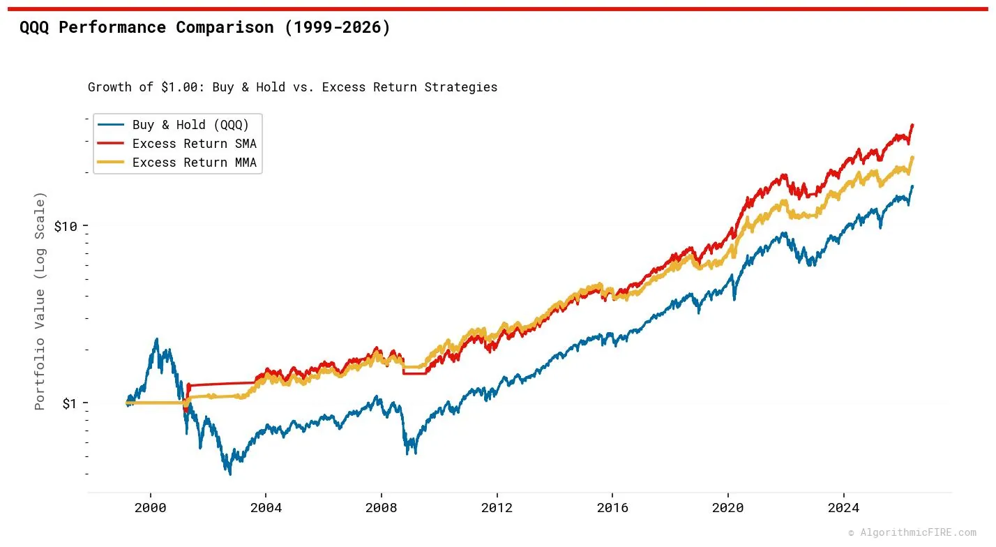
The chart above is a visual representation of what we are aiming to achieve. Shown (blue) is the normalized price (starting value = 1.0) for QQQ (Nasdaq 100 index ETF), and (yellow) the gain from trading using a trend following strategy. As the chart illustrates, the trend-following strategy effectively sidestepped the worst of the dot-com bubble and the 2008 Financial Crisis. While out of the market, the portfolio continued to generate modest returns by pivoting into U.S. Treasuries.

In this case, the strategy resulted in substantially higher overall gain, with much less volatility. Consider the higher gain of the trend following results an anomaly; you will usually give up some gains in order to have the downside protection—a phenomenon we’ll explore across more ETFs below.

Examination of Trend Following Methods

With that understanding of what we hope to achieve, we present results from three trend-following strategies:

• Excess Return (SMA): This approach compares the moving average of a security against the moving average of a "risk-free" benchmark (using the 3-Month U.S. Treasury yield, DGS3MO). If the security is outperforming the benchmark on a trend basis, it triggers a buy signal. Otherwise, it triggers a sell and sweeps the proceeds to cash. This is a binary strategy (either 100% invested or 100% in cash).
• Excess Return (MMA): An ensemble version of the Excess Return strategy that uses multiple moving averages to scale in and out of the security. Instead of an all-or-nothing approach, the portfolio holds varying percentages (0%, 33.3%, 66.7%, or 100%) in the security, with the remainder swept to cash earning interest. This strategy offers smoother transitions but generates more trades.
• Excess Return (MMA CA): Built on the exact same ensemble logic and signal parameters as the Excess Return MMA strategy. However, instead of sweeping out-of-market capital to a static cash interest rate, it dynamically rotates capital among a high-liquidity, defensive basket of ultra-short Treasury and floating-rate ETFs (FLOT, SHV, BIL) based on their momentum and trend signals. This serves as a "Cash Alternative" sleeve to optimize defensive yields while strictly managing duration risk (see Addendum: Dynamic Cash Alternatives below).
• Moving Average (A.K.A. The Golden Cross/Death Cross): A classic trend-following strategy using the 50-day and 200-day simple moving averages. A buy is triggered when the 50-day MA climbs above the 200-day MA (Golden Cross), and a sell is triggered when it breaks below (Death Cross).

The standard strategies invest in U.S. 3-Month Treasuries when not holding the target security, while the Cash Alternative (CA) variant dynamically rotates across defensive ETFs during cash-sweep periods.

Strategy Styles: Investing vs. Trading

Each strategy in our analysis is backtested under one of two execution styles:

• Investing Style: Uses longer-term trends to minimize transaction frequency, reducing portfolio turnover and potential tax drag in taxable accounts. The statistics and charts throughout this post are based on the Investing Style.
• Trading Style: Uses shorter-term trends for faster responsiveness. While it reacts more rapidly to market turns, it generates significantly more trades. Up-to-date results for both styles across all assets are available on the live Dashboard.

We are not including the tax impact of capital gains in this analysis. There are three reasons for this:

1. The focus of this analysis is downside protection, not tax efficiency.
2. Retirement funds are frequently held in tax-advantaged accounts.
3. The tax impact is complex to calculate and would require additional assumptions.

That said, the impact may be non-zero, and we address this in a separate post on capital gains tax impacts, which is particularly relevant if you hold significant assets in taxable accounts.

It should be noted that these are just three strategies in the general realm of trend following. There is a limitless range of possible strategies using different timeframes, moving average types (simple, exponential, weighted), stop-losses, and cash sweeps.

Quick-Buy and Stop-Loss Solve Reaction Time Problems

Standard moving averages are slow to react. To solve this and prevent being left behind during V-shaped recoveries or caught in rapid crashes, we incorporate two supplementary algorithms:

• Quick-Buy: If a security closes higher for seven consecutive trading days, the algorithm triggers a buy signal regardless of the longer-term moving averages. (This transitions to a normal buy signal if the averages eventually cross, and sells on a 5% drop while in the quick-buy state.)
• Stop-Loss: An automatic risk-mitigation tool that triggers a sell if the security drops below a predetermined threshold (varying by asset class to account for historical volatility), protecting the portfolio from rapid, vertical selloffs.

That is the extent of the algorithms:

• Buy/sell based on moving average trends.
• Buy when a security is consistently advancing (Quick-Buy).
• Sell a security immediately if it drops significantly and too fast for the moving averages to react (Stop-Loss).

Performance

To validate these strategies, we backtested all three algorithms across the 106 stock ETFs in our coverage universe, comparing their performance directly to a traditional buy-and-hold approach. The testing period for each fund spans its entire available history, adjusted for the lead-in time required to calculate the moving averages.

We will evaluate the strategies using three key metrics:

• Maximum Drawdown: The largest peak-to-trough drop in a portfolio's value, showing the worst potential loss.
• CAGR (Compound Annual Growth Rate): The average yearly rate of return.
• Sharpe Ratio: A metric of risk-adjusted return (reward per unit of volatility). A higher Sharpe ratio indicates a more efficient portfolio.

Maximum Drawdown

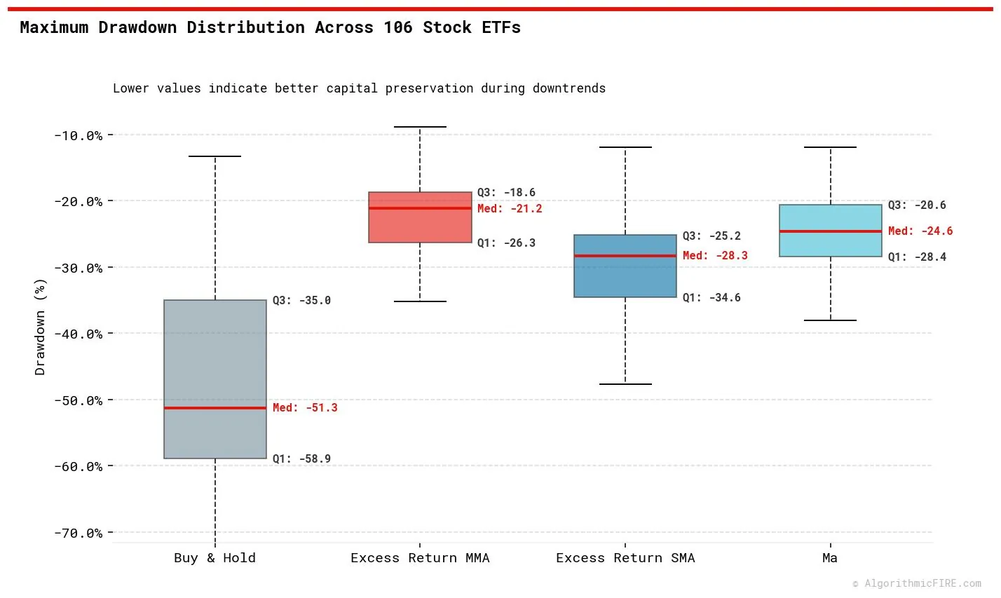
For each ETF, using each strategy, the maximum drawdown was determined and is charted above. Drawdowns are significantly reduced using any of the trend-following strategies:

• The median drawdown is -51.3% for buy-and-hold, but drops to -28.3% for Excess Return SMA, -21.2% for Excess Return MMA, and -24.6% for the Moving Average strategy.
• First quartile (worst 25th percentile) drawdowns were: buy-and-hold (-58.9%), Excess Return SMA (-34.6%), Moving Average (-28.4%), and Excess Return MMA (-26.3%).
• During the Great Financial Crisis (GFC), buy-and-hold experienced a -60.7% drawdown if you held QQQ, compared to just -29.2% for the Excess Return SMA strategy and -20.9% for the Excess Return MMA strategy.

CAGR

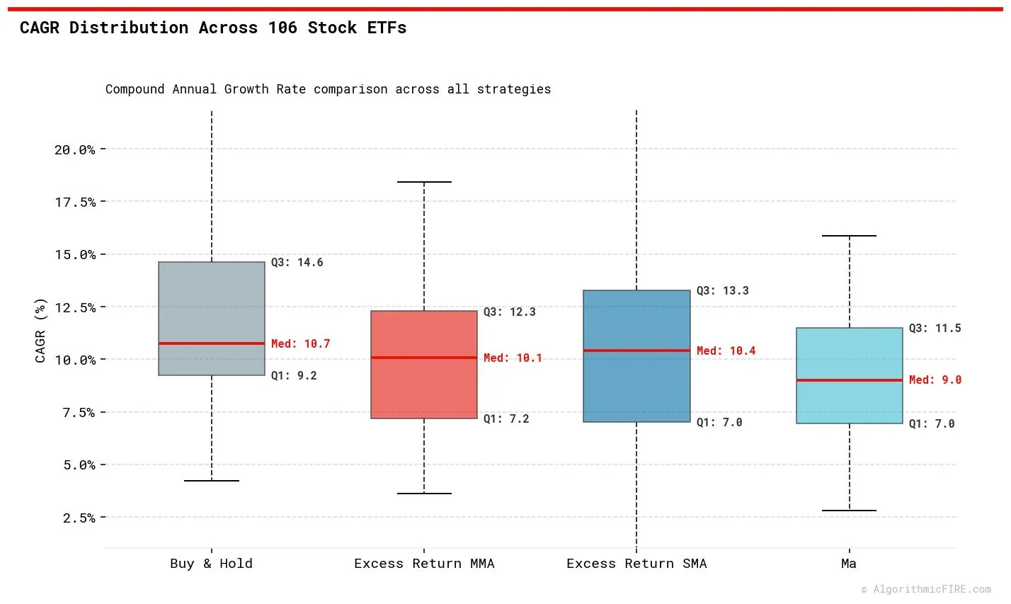
For each ETF, using each strategy, the CAGR was determined and is charted above:

• Buy-and-hold achieved a median CAGR of 10.7%.
• The Excess Return SMA strategy closely matched this at 10.4% median CAGR, while the Excess Return MMA strategy followed at 10.1%.
• The Moving Average strategy trailed both at a 9.0% median CAGR.

This aligns with our expectations: trend following behaves like portfolio insurance. While insurance significantly reduces drawdowns (risk), it comes at a minor cost to the compound annual growth rate (CAGR), especially in the Moving Average strategy.

Sharpe Ratio

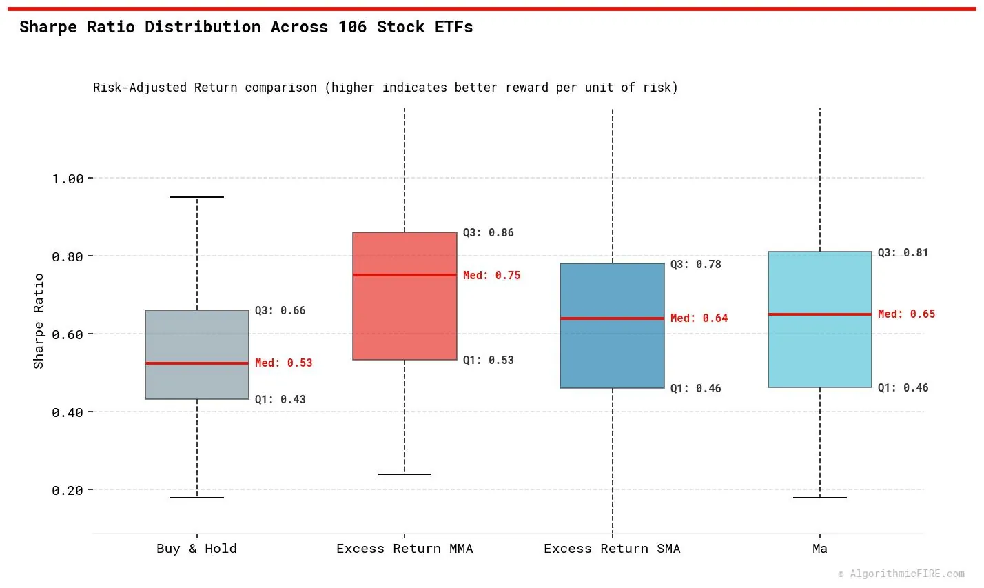
The Sharpe ratio indicates that the reduction in drawdowns is well worth the minor drag on returns:

• The median Sharpe ratio for buy-and-hold is 0.53.
• All three trend-following strategies achieved substantially higher median Sharpe ratios: 0.64 for Excess Return SMA, 0.65 for Moving Average, and 0.75 for the ensemble Excess Return MMA.
• This demonstrates that trend following significantly improves risk-adjusted returns compared to buy-and-hold.

Asset Class Suitability: Why Indices and Fixed-Income Excel

While we provide comprehensive backtests on our live dashboard across a wide range of asset classes—including bond ETFs, stock ETFs, individual equities, and commodities—the quantitative reality is that trend-following does not perform equally across all categories:

• Fixed-Income (Bonds): Trend-following performs exceptionally well on bond ETFs. Fixed income is highly sensitive to macroeconomic interest rate regimes, which tend to persist in multi-year macro cycles (bull and bear bond markets). With lower natural volatility, whipsaws are minimal, and trend-following shields capital cleanly from prolonged rate hikes.
• Equity Index ETFs: Diversified stock indices (like SPY or QQQ) represent broad economic growth trends. Diversification naturally smooths out individual company news, making these index ETFs highly responsive to macro-economic momentum.
• Individual Stocks: Trend-following is far less effective here. Individual stocks are subject to high idiosyncratic volatility, corporate events, and "gap risk" (e.g., earnings releases causing a stock to gap down 20% overnight). Trend algorithms get whipsawed frequently by this corporate noise, cutting winners too early and taking sudden gap-down losses.
• Commodities: Assets like Gold, Oil, or Agriculture are highly cyclical and prone to sudden supply shocks and extended periods of range-bound mean-reversion. Trend-following in commodities often suffers from severe whipsaw drag during choppy, sideways markets.

We have included individual equities and commodity ETFs on our platform primarily to satisfy the common query, "but how does this perform on X?" However, for systematic retirement protection and safe withdrawal security, the data strongly favors sticking to diversified index and fixed-income ETFs.

To support this flexibility, the platform's custom portfolio builder allows you to incorporate these assets into your personal allocations while electing a passive, buy-and-hold strategy for these specific sleeves instead of forcing a trend-following overlay.

Takeaways

• Trend following systematically reduces the probability of holding securities into a significant downturn.
• While the reduction in risk can come at the expense of a minor reduction in CAGR, the risk-adjusted returns (Sharpe ratios) are significantly superior to buy-and-hold.
• The ensemble Excess Return MMA strategy offers the best risk-adjusted profile (highest median Sharpe ratio at 0.75) and lowest median drawdown (-21.2%).

A Practical Example

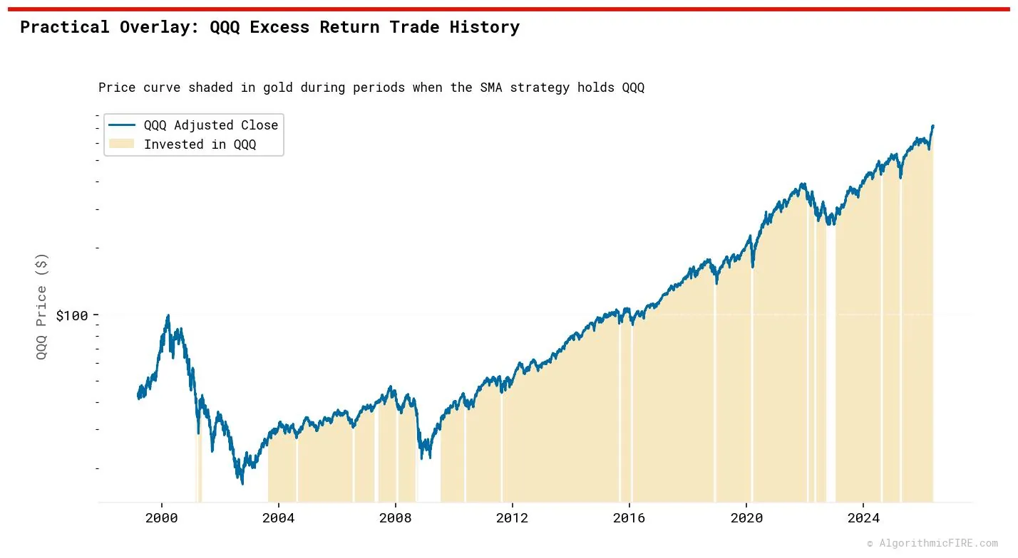
The chart above shows the QQQ price history with overlays indicating the periods when the Excess Return SMA strategy was invested in the market (shaded in gold).

As illustrated, the strategy successfully exited QQQ, sidestepping the worst of the dot-com crash and the 2008 Financial Crisis, while capturing the subsequent bull runs. The compound effect of avoiding these major downturns—while continuing to accumulate interest income during down cycles—is what drives the substantial wealth outperformance shown in the cumulative growth chart (Chart 1) at the beginning of this post.

Addendum: Trading Style Comparison

While the main analysis of this post focuses on the Investing Style (designed for long-term builders, using longer-term trends to minimize transaction frequency and turnover), our platform also backtests a more active Trading Style. This style uses shorter moving averages to react more rapidly to market turns.

Below is the statistical performance of the Trading Style across the stock ETF universe:

Maximum Drawdown (Trading Style)

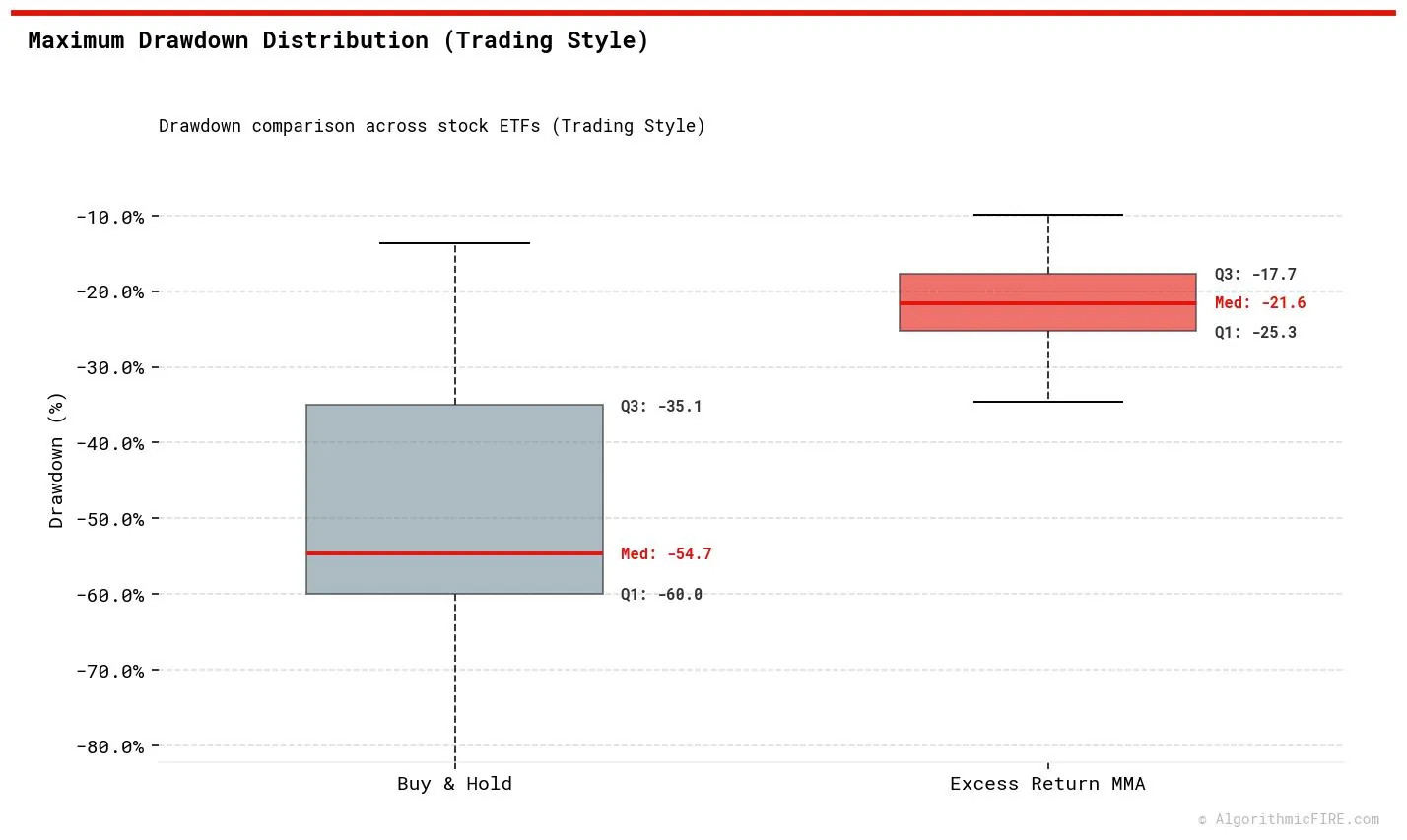The median maximum drawdown for the Trading style is -21.6% (compared to -21.2% for the Investing style).

CAGR (Trading Style)

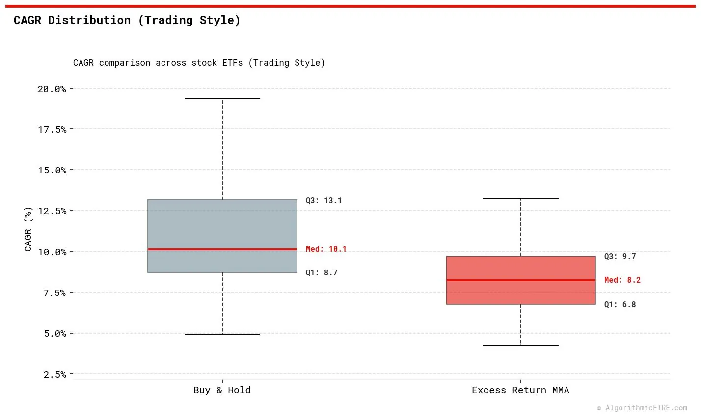The median CAGR is 8.2% (compared to 10.1% for the Investing style).

Sharpe Ratio (Trading Style)

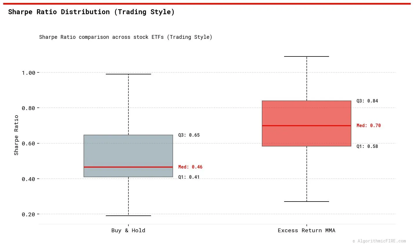The median Sharpe ratio is 0.70 (compared to 0.75 for the Investing style).

Core Comparison Summary

The data illustrates a key trend-following lesson: faster responsiveness is not always better. While the Trading Style exits positions slightly quicker during sharp declines, the increased frequency of trades leads to "whipsaws" (buying and selling on short-term market noise). This friction drags the median CAGR down to 8.2% (vs. 10.1% for the Investing style) and lowers the risk-adjusted return (Sharpe ratio of 0.70 vs. 0.75), while yielding virtually identical drawdown protection.

Utility of the Trading Style

While the long-term historical averages favor the Investing Style, the Trading Style serves a specific utility for investors prioritizing rapid risk mitigation. In periods of high market volatility or swift, severe market downturns, the shorter moving averages trigger defensive cash sweeps significantly faster, protecting capital early in the sell-off. The tradeoff, however, is that you must be willing to accept more frequent false signals ("whipsaws") and higher transaction turnover in exchange for this response time.

Addendum: Dynamic Cash Alternatives (Excess Return MMA CA)

In our standard strategies, out-of-market capital is swept into a cash proxy pegged to the 3-Month U.S. Treasury yield. However, in low or shifting interest rate environments, holding raw cash or standard short-term treasuries can leave yield on the table or introduce mild interest rate risk.

To address this, we developed a dynamic cash management option: Excess Return MMA CA (Cash Alternative). This strategy executes the identical ensemble entry and exit signals on the primary asset as the Excess Return MMA strategy, but manages the cash sleeve dynamically by rotating capital among a high-liquidity defensive basket of three ETFs:

1. FLOT: iShares Floating Rate Bond ETF (Floating-rate corporate debt yielding credit spread premium)
2. SHV: iShares Short Treasury Bond ETF (0-12 Month U.S. Treasuries)
3. BIL: SPDR Bloomberg 1-3 Month T-Bill ETF (Ultra-short Treasury bills)

Design Note: We analyzed versions of the CA sleeve that included medium-term and corporate bond funds (BNDX, VCSH, VTIP). However, quantitative audits revealed that during stock market drawdowns, these funds introduced duration risk and credit risk, resulting in capital losses at the exact moment the strategy was seeking defensive shelter. To prevent this, the CA sleeve is strictly restricted to near-zero duration assets, ensuring capital preservation matches standard cash.

Cash Alternative Sleeve Rules

On the second trading day of each month, the cash sleeve dynamically selects the optimal defensive ETF:

• Trend Filter: Each candidate ETF is evaluated using a simple trend filter—its price must be above its 25-day moving average.
• Momentum Ranking: Among the ETFs that pass the trend filter, the strategy ranks them by their 54-day absolute momentum (return over the lookback period) and selects the asset with the strongest performance.
• Defensive Fallback: If all candidate ETFs fail the trend filter, the sleeve defaults to BIL as the baseline cash holding. For historical backtesting dates prior to BIL's launch on May 25, 2007, the system seamlessly falls back to standard 3-Month Treasury interest rates (DGS3MO), which are logged in our reports as "CASH".

By utilizing a 54-day momentum lookback and rebalancing on the second trading day, the strategy avoids ex-dividend date clustering noise. This allows the portfolio to capture higher yields from corporate credit spreads (FLOT) or short-term rates (SHV, BIL) during stable environments, while automatically retreating to T-bills when rates or credit markets show stress.

Tax & Execution Friction Note: Because the CA sleeve dynamically rotates between ETFs on a monthly basis, it generates frequent transaction events:

• Transaction Drag & Bid/Ask Spreads: For these specific ETFs (FLOT, SHV, BIL), transaction costs are negligible. Because they are highly liquid institutional-grade funds, they trade with extremely tight bid/ask spreads (typically $0.01 per share, or under 0.02% friction) and zero commission on modern brokerages. The cumulative annual drag of these rotations is under 0.15%, which is easily offset by the yield premium.
• Tax Consequences: In a taxable brokerage account, these monthly rotations generate short-term capital gains tax liabilities and reporting friction. This tax drag can quickly consume the marginal yield advantage. Consequently, the Excess Return MMA CA strategy is recommended for tax-advantaged accounts (such as IRAs or 401ks), while the standard Excess Return MMA strategy (which sweeps to static interest-bearing cash) is generally more practical for taxable accounts.

Understanding the Backtest Trade Logs

When exploring the interactive simulations on the dashboard, each asset and portfolio features a detailed Trade History log table. To understand the output, keep these three trade types in mind:

• Completed Trades: Standard trades showing when the system bought an asset (entry) and sold it (exit) based on moving average signal crossovers.
• Open / Mark-to-Market Trades: If the system is currently holding an asset at the end of the backtest simulation, the final position is marked to market using the latest available price so that all cumulative gains are accounted for.
• Interest Trades: When the system is out of the market (holding cash/yield), these entries record the yield/interest income accrued over the out-of-market duration. For standard strategies, this tracks the Treasury rate; for CA strategies, it tracks the active defensive ETF (like SHV or FLOT).

Access to All Results, Updated Daily

If you enjoyed this post and would like to follow along, we update these simulations daily across hundreds of assets on our interactive Dashboard.

Interactive results include:

• Results for the 100+ largest stock ETFs
• Results for the 100+ largest bond ETFs
• Results for the 100+ largest individual stocks
• Customizable multi-asset model portfolio builders