📌 Summary & Key Takeaways
- 5.0% SWR Failures Are Concentrated in 2 Major Inflation & Stagflation Regimes: Across 816 rolling 30-year monthly cohorts (50% S&P 500 / 50% 5-Year Treasuries from 1928 to 1995), a 5.0% SWR shows a 74.1% overall success rate (605 of 816 cohorts survived). Every single failure cluster is concentrated in the 1929 Great Crash / 1936–1940 Great Depression echo and the 1959–1973 stagflation era.
- Stagflationary Inflation Is More Destructive Than Market Crashes: The 1960s cohort bankruptcies were not triggered by sudden equity crashes — nominal returns appeared stable. The failure mechanism was real return drag: inflation eroded purchasing power while nominal returns stagnated, depleting portfolios within 19 to 30 years.
- Failures Occur Deep Into Retirement (Years 19–30): Every single 5.0% SWR bankruptcy occurred at Year 19 or later (with over 80% failing in Years 21–30). By Year 15 (Month 180), the median failing portfolio had already declined to roughly 35% of its starting real value — providing a critical window to adjust spending or generate supplemental income before running out of capital.
Historical Success Rates & Failure Regimes
In my previous analysis of Safe Withdrawal Rates (SWR), I modeled baseline survival math across generic return and volatility distributions. But I wanted to test what happens when we stress-test higher withdrawal rates against actual U.S. market history starting in 1928 across 816 rolling 30-year monthly cohorts.
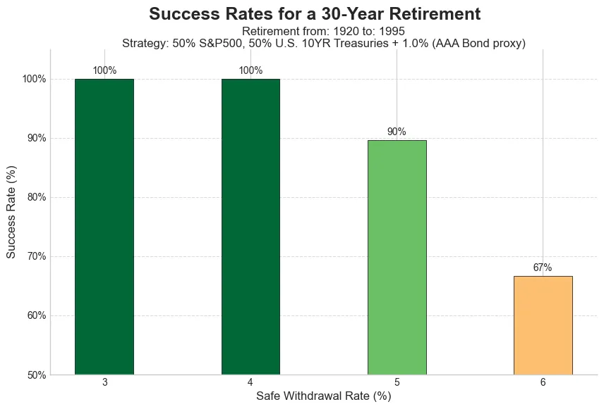
This chart models historical 30-year survival rates for 3.0%, 4.0%, 5.0%, and 6.0% withdrawal rates applied to a 50/50 stock/bond portfolio (50% S&P 500 and 50% 5-Year Intermediate Treasuries).
While a 3.0% SWR achieved a 100.0% survival rate and a 4.0% SWR achieved 99.8% (814 of 816 cohorts), a 5.0% SWR survived in 74.1% of starting 30-year monthly cohorts (605 of 816 cohorts). But what does that ~26% failure rate look like in real dollars, and when do those bankruptcies hit?
Portfolio Returns: Nominal vs. Real Purchasing Power
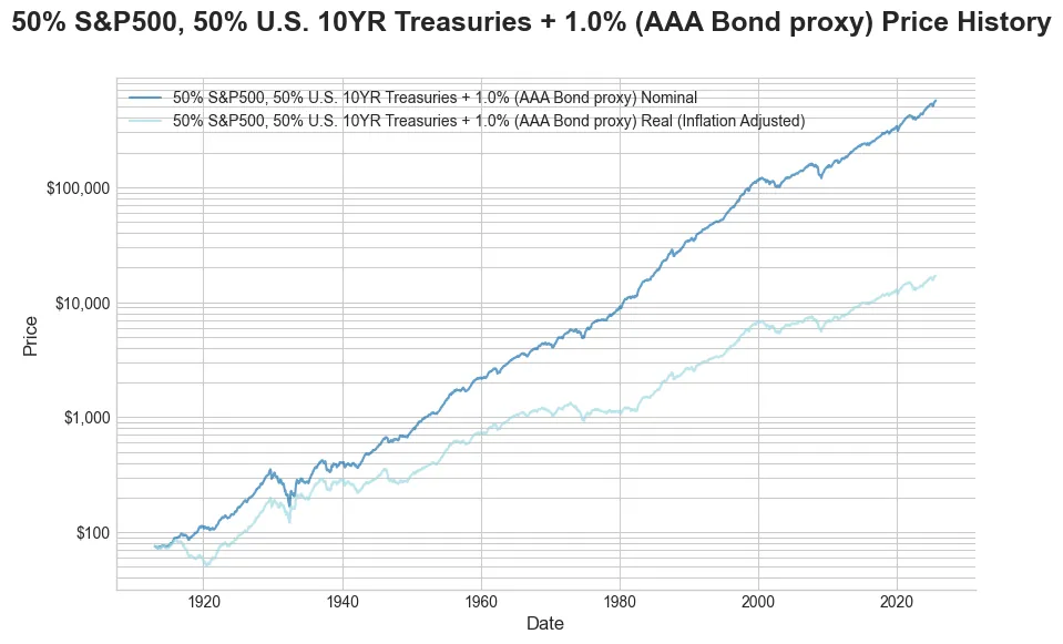
To model decumulation accurately, we have to look at real (inflation-adjusted) returns. The portfolio modeled here uses 50% S&P 500 and 50% 5-Year Intermediate Treasuries.
The Stealth Drag of Inflation
During the 1960s and 1970s, nominal portfolio balances appeared to drift upward on paper. But real purchasing power was flat to declining. Inflation matched or exceeded nominal portfolio growth, silently eroding the principal needed to sustain annual inflation-adjusted withdrawals.
Failures Are Clustered, Not Random
When I mapped failing 30-year monthly cohorts onto annual real return histories, a striking pattern emerged:
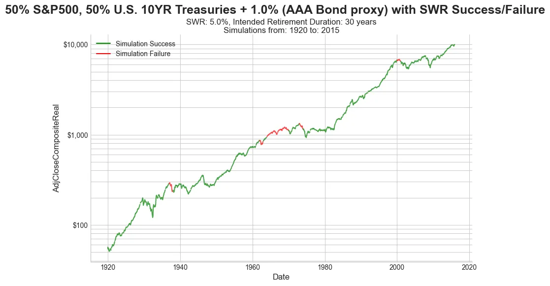
Retirement failures were not randomly distributed across time. Every single bankruptcy was concentrated into distinct starting market clusters:
- Late 1920s & 1930s (1928–1930, 1935–1940): Wall Street Crash of 1929 and post-Depression echo crash with stagnant real yields.
- Mid-1950s to Early 1970s (1955–1956, 1959–1973): Persistent 1960s–1970s stagflation and real return drag.
Failure Breakdown Math
- Failing Cohort Months: 211 failing monthly cohorts out of 816 (1928-12 to 1930-09, 1935-11 to 1940-04, 1955-12 to 1956-08, and 1959-01 to 1973-07).
- Years to Depletion: Ranged from 19.4 to 29.9 years.
- Over 80% of failures occurred in Years 21–30.
- 100% of failures occurred at Year 19 or later.
Because depletion happened late in retirement, early account balances looked deceptively safe during the first decade.
Anomaly Case Studies: The Mechanism of Failure
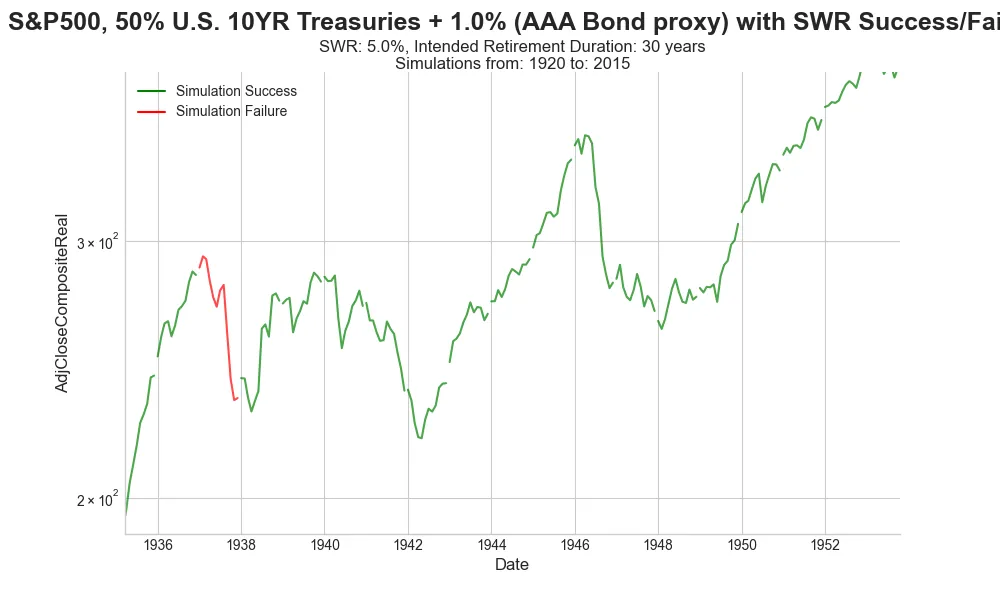
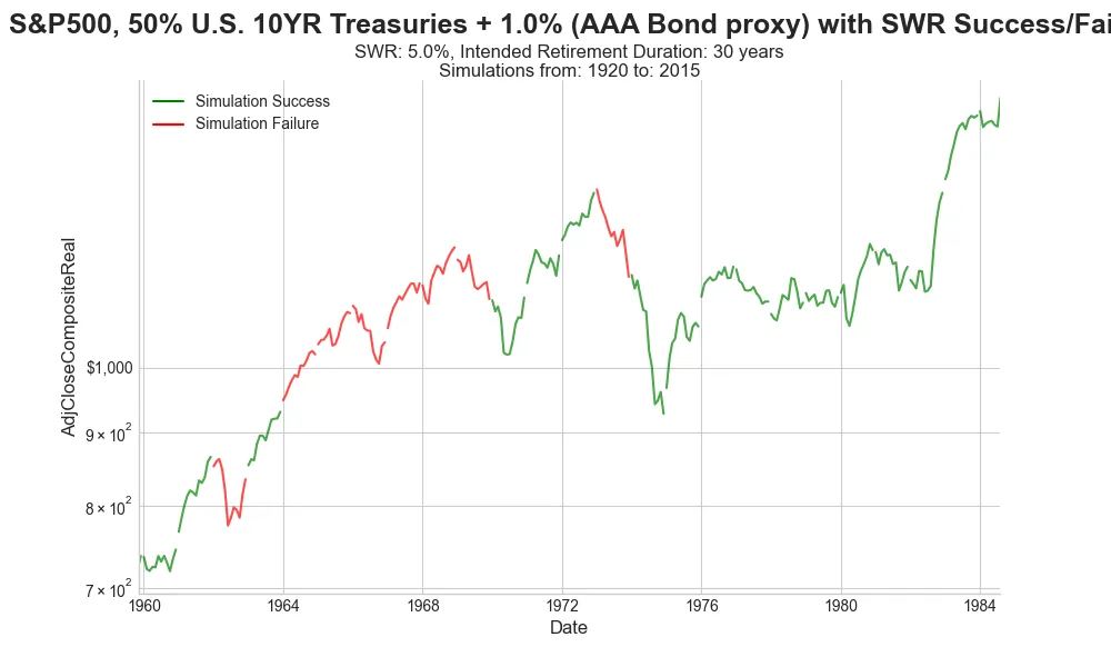
Examining the trajectory curves above reveals that bankruptcy occurs when a retirement starts immediately prior to an extended multi-year stretch of near-zero real returns.
The Depletion Trajectory: How Bankruptcies Unfold
"How did you go bankrupt? Two ways. Gradually, then suddenly."
— Ernest Hemingway, The Sun Also Rises
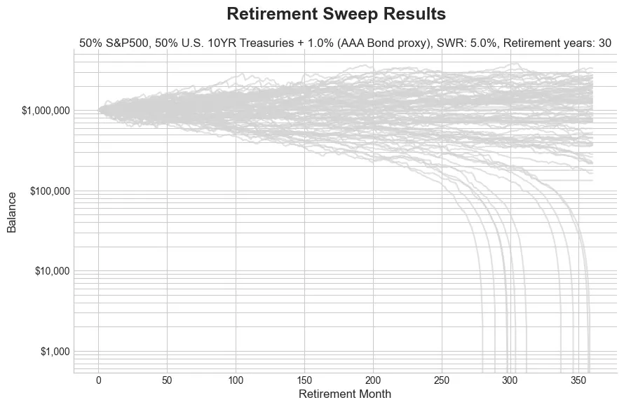
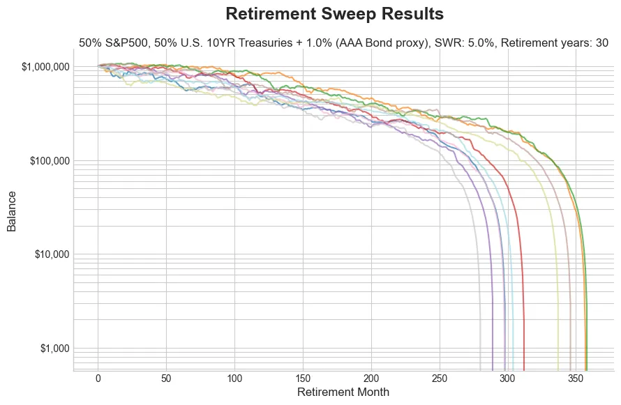
Comparing all 816 historical monthly cohort trajectories (top) against failing cohorts only (bottom) highlights an important diagnostic benchmark:
By Year 15 (Month 180), the median failing portfolio had already declined to roughly 35% of its starting real purchasing power (83% of failing cohorts were below 50%). This provides a 15-year early warning window for retirees to adjust spending before capital depletion accelerates.
Pushing the Limit: What Happens at a 6.0% SWR?
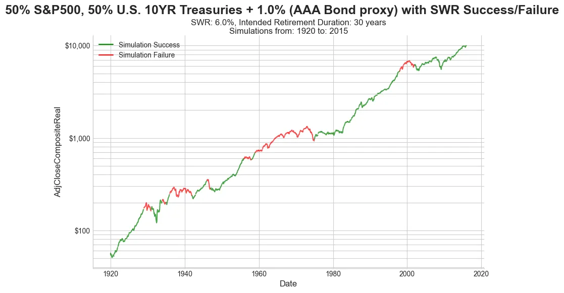
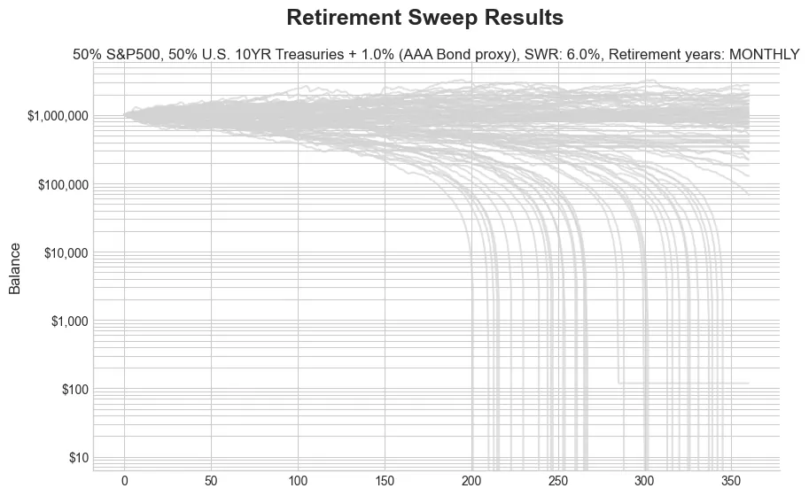
When I increased the withdrawal rate to 6.0%:
- The overall historical success rate dropped from 74.1% down to 52.1% (425 of 816 monthly cohorts survived).
- Failure clusters expanded significantly across starting cohorts.
- Depletion timelines accelerated, with account balances running out as early as Year 15.
Best Case Scenarios: Portfolio Accumulation Surprises
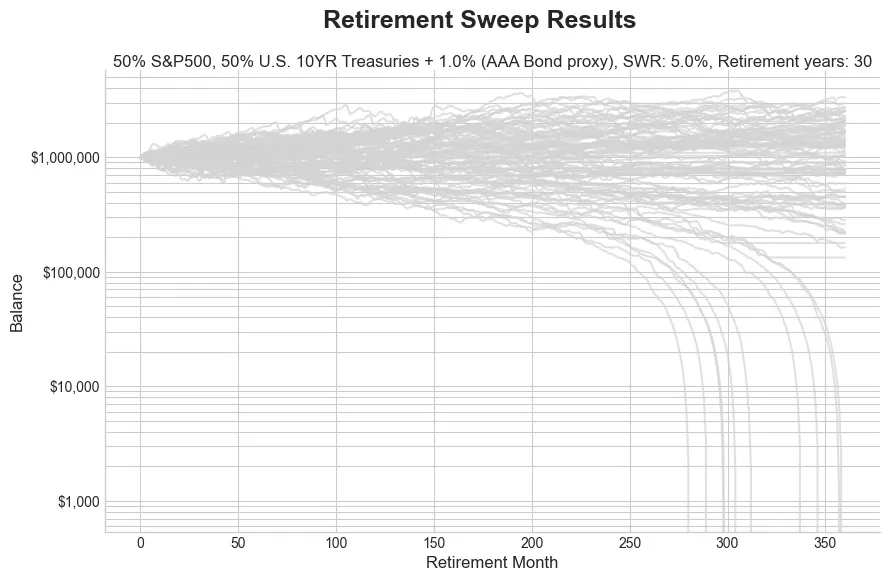
While failing runs ran out of capital late in retirement, the top 25% of surviving historical runs saw account balances compound to $1.6M–$4.4M+ by Year 30. A conservative withdrawal rate paired with strong early market returns creates substantial upside wealth.
Key Takeaways
- Failures Occur Deep in Retirement: Depletion typically hits in Years 19–30, when returning to full-time work is least feasible.
- Track Real Returns, Not Nominal Balances: Multi-year stretches of near-zero real returns are far more destructive to withdrawal survival than short, sharp market crashes that recover quickly.
- Use Year 15 as an Early Warning Checkpoint: If portfolio real balance drops below 50% of starting value by Year 15, it's a strong signal of a failing trajectory — reduce spending or supplement income to ride out the economic cycle.
- Modest Adjustments Restore Resilience: Reducing a withdrawal rate from 5.0% to 4.0% restores 99.8% historical survival across all 816 monthly 30-year cohorts since 1928.
Methodology & Bengen Benchmark Comparison
💡 Methodology Callout: Monthly Cohort Density vs. Bengen Benchmark & CPI Adjustments
- High-Density Monthly Starting Cohorts: Unlike William Bengen's classic 1994 paper ("Determining Withdrawal Rates Using First-Day-of-the-Year Data"), which evaluated 50 annual cohorts starting on January 1st of each year, this simulation runs a high-density quant sweep of 816 rolling 30-year monthly cohorts starting on the 1st of every month from January 1928 to December 1995.
- Annual CPI Step-Up Withdrawal Mode (
WITHDRAWAL_MODE_ANNUAL_CPI_STEP): To model realistic retiree budgeting, withdrawals are modeled using annual CPI step-ups. A retiree sets a fixed nominal monthly withdrawal amount for Months 1–12 based on the initial withdrawal rate (e.g. 5.0% / 12 = $4,166.67/mo on a $1M portfolio). At Month 13 (and every 12 months thereafter), the monthly withdrawal amount steps up by the trailing 12-month CPI inflation rate.- Comparison with Continuous Real Decumulation (
WITHDRAWAL_MODE_CONTINUOUS_REAL): Continuous real decumulation adjusts the monthly withdrawal amount every single month based on that exact month's CPI. In practice, annual CPI step-ups generate identical survival success rates over 30-year horizons while capturing the real-world friction of annual budget adjustments.