📌 Summary & Key Takeaways
- SWR Translates Portfolio Size Into Annual Income: The Safe Withdrawal Rate defines the percentage of starting capital you can withdraw annually (adjusted for inflation) without running out of money over a 30-year retirement. At a 4.0% SWR benchmark, a $1,000,000 portfolio yields $40,000/year in inflation-adjusted income.
- Volatility Drag Is Why SWR Is Lower Than Average Returns: Although the S&P 500 averages a 7.5% historical real return, in my 500 Monte Carlo simulations at a 4.0% SWR, a 100% stock portfolio suffered 30 failures out of 500 (6.0% failure rate / 94.0% success rate) using the historical returns (7.5%) and volatility (14.8%) of the S&P 500.
- Diversification & Volatility Control Reduce Depletion Risk: By adding intermediate Treasuries to lower volatility, my simulated mixed portfolio (60/40) maintained a 96.4% success rate (18 failures out of 500) while generating a $1,603,330 median ending balance at a 4.0% withdrawal rate.
When I design decumulation models for early retirement, the core question that needs answered is: "What withdrawal rate can my portfolio sustain without running out of capital?"
What Is SWR? Safe Withdrawal Rate Meaning Explained
The Safe Withdrawal Rate (SWR) is the percentage of your initial retirement portfolio that you withdraw in Year 1, with that dollar amount subsequently adjusted for inflation each year, designed to maintain portfolio solvency over a 30-year horizon.
💡 Methodology Note: This analysis relies on Monte Carlo simulations drawn from parameterized real return (\mu) and volatility (\sigma) distributions. It models theoretical distribution risk across different return profiles rather than backtesting against exact historical market sequences (such as the Trinity Study and Bengen's original work).
💡 Test Your Plan: Calculate your personal withdrawal capacity using my interactive Safe Withdrawal Rate Calculator or explore defensive allocations in the Model Portfolios Hub.
The 4% Benchmark & The Bengen Framework
Financial planner William Bengen established the widely cited 4% rule (SWR of 4.0%) by backtesting historical U.S. stock and bond data through severe economic periods like the Great Depression and the 1970s stagflation shock. Bengen later updated his research to suggest a 4.5% baseline under specific portfolio conditions.
Bengen's specific portfolio: 50% S&P 500, 50% Intermediate Term Government Bonds. The citied 4% rule meant that there were 0 failures for any given 30 year retirement period in the historical data that he backtested (1926-1992).
References & Background:
Why Is SWR Significantly Lower Than S&P 500 Average Returns?
Investors frequently ask why a sustainable withdrawal rate is 4.0%–4.5% when the historical real return of the S&P 500 is roughly 7.5%.
If annual market returns were constant with zero variability, an investor could safely withdraw 7.0% or more each year. But real-world markets fluctuate violently. When high return volatility is combined with annual withdrawals, Sequence of Returns Risk permanently destroys capital during drawdowns.
Real vs. Nominal Returns: What Matters for Retirement
- Nominal Return: The raw percentage gain reported on account statements before inflation, taxes, or fees.
- Real Return: The actual growth in purchasing power (
Nominal Return - Inflation).
Real Returns in My Simulation Models
Throughout this presentation, all financial figures and analyses, including withdrawal rates and portfolio values, are expressed in terms of real returns. This means all dollar amounts are adjusted for inflation and represent constant purchasing power, equivalent to today’s money.
This approach is crucial for retirement planning because it provides a clearer, more accurate picture of what your money can truly purchase in retirement. By accounting for inflation, we ensure our discussions reflect actual buying power, allowing for more realistic and actionable financial strategies.
The Role of Standard Deviation (Return Volatility)
Standard Deviation (STDEV) measures how widely annual returns scatter around their mean value. In a standard normal distribution:
- 68.2% of annual returns fall within ±1 STDEV of the mean.
- 95.4% of annual returns fall within ±2 STDEV of the mean.
- 99.7% of annual returns fall within ±3 STDEV of the mean.
High standard deviation creates wide return swings, increasing the frequency of early market crashes during retirement.
Mechanics of My SWR Simulation Engine
To evaluate sustainable withdrawal boundaries, I built a 2D Monte Carlo simulation engine:
- Parameter Grid: Select real mean return (1% to 10%) and return STDEV (0% to 25%).
- Trajectory Generation: Execute 500 independent 30-year retirement runs for each grid coordinate under fixed inflation-adjusted annual withdrawals.
- Solvency Evaluation: Count a run as Success if portfolio balance > $0 at Year 30, and Failure if capital is depleted before Year 30.
SWR Simulation Heatmaps: 4.0% vs. 6.0% SWR
4.0% SWR Success Map
Below is the contour heatmap generated from my code evaluating 500 retirement runs per grid cell at a 4.0% withdrawal rate:
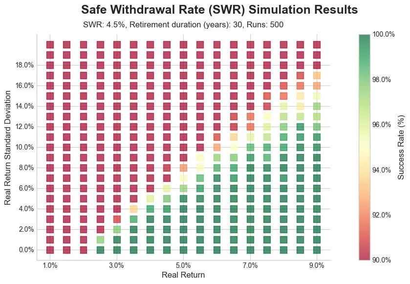
- Red zones represent parameter combinations with high failure rates.
- Green zones represent combinations with high solvency rates (>95%).
6.0% SWR Success Map
When I raise the withdrawal rate from 4.0% to 6.0%, the safe envelope shrinks drastically:
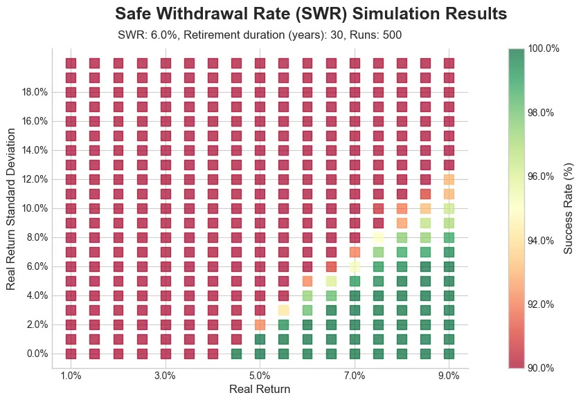
At a 6.0% SWR, maintaining portfolio solvency requires either an unrealistic 7.0%+ real return at near-zero volatility, or unrealistic asset growth.
Mapping Asset Classes onto the 4.0% SWR Envelope
Below, I overlaid historical asset class profiles onto the 4.0% SWR success map:
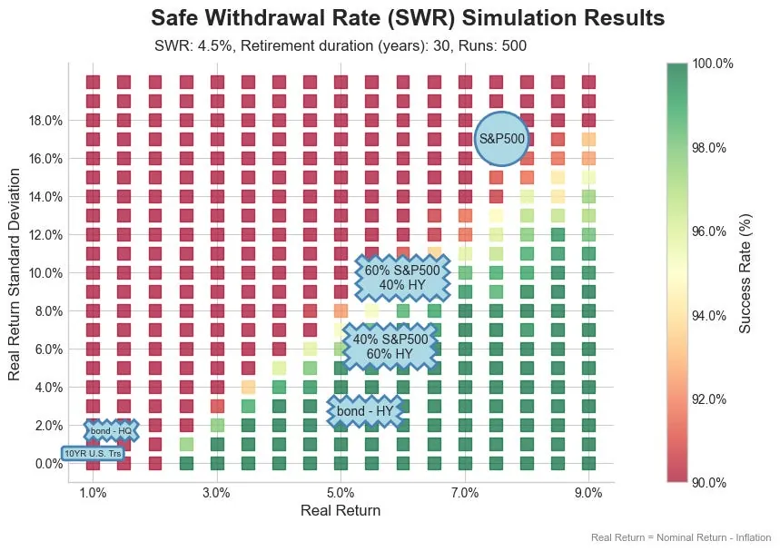
Historical Asset Parameters (Real Returns, 1953–2026 Modern Era):
- High Quality Corporate Bonds (Moody's AAA 20Y): 2.5% Real Return | 7.6% STDEV (Moderate stability, low inflation-adjusted return)
- Investment Grade Corporate Bonds (Moody's BAA 20Y): 3.5% Real Return | 7.1% STDEV (Higher credit spread yield)
- 5-Year Intermediate Treasuries: 1.6% Real Return | 4.7% STDEV (Risk-free principal anchor)
- S&P 500 (100% Stocks): 7.5% Real Return | 14.8% STDEV (High long-term real growth, higher sequence-of-returns volatility)
- Mixed Portfolio (60% S&P 500 / 40% 5-Yr Treasuries): 5.4% Real Return | 9.4% STDEV (Optimized return/volatility balance)
30-Year Trajectory Analysis: Mixed Portfolio vs. 100% Stocks
Mixed Portfolio (60/40) at 4.0% SWR
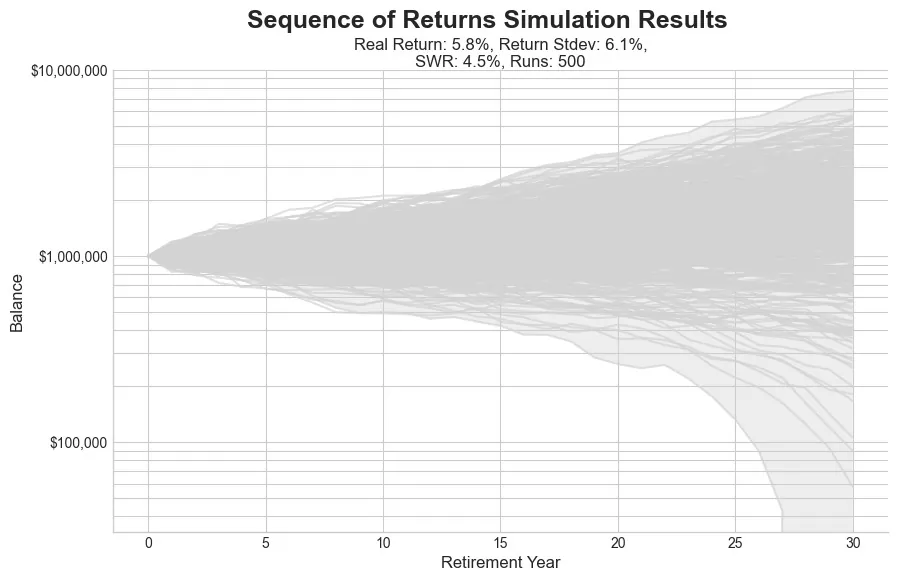
- Real Mean: 5.4% | STDEV: 9.4%
- Failures: 18 out of 500 (3.6% failure rate / 96.4% success rate)
- Median Final Balance: $1,603,330
By dampening return volatility to 9.4% relative to 100% equities, the mixed portfolio achieves high solvency (96.4% success rate) while generating substantial median capital growth.
100% Stock Portfolio at 4.0% SWR
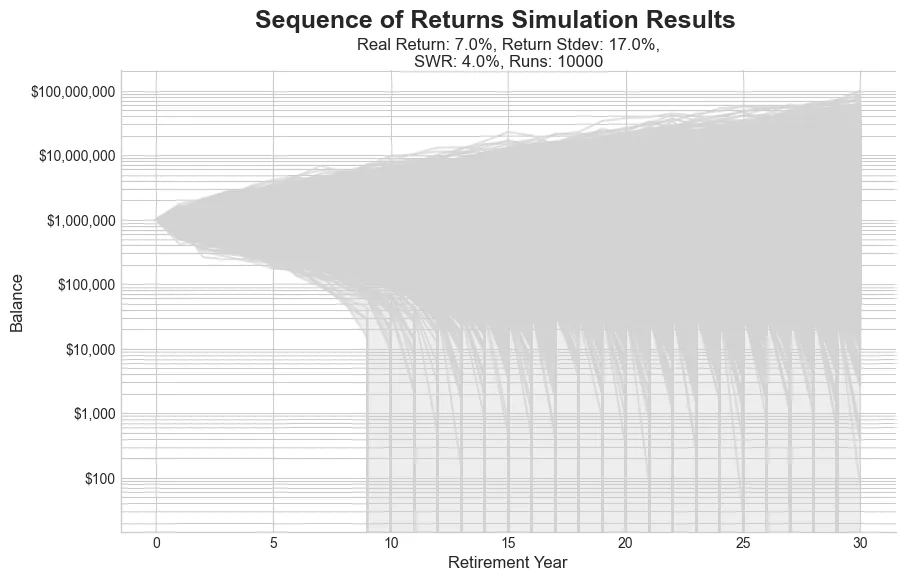
- Real Mean: 7.5% | STDEV: 14.8%
- Failures: 30 out of 500 (6.0% failure rate / 94.0% success rate)
- Median Final Balance: $2,916,412
Despite delivering a higher average real return (7.5% vs 5.4%), the 100% stock portfolio experienced wider return dispersion and nearly double the failure count (30 vs 18) due to its 14.8% return volatility.
Key Takeaways
- Volatility Management Trumps Return Chasing: Reducing return volatility is more critical for decumulation survival than maximizing raw returns. A lower-yielding, lower-volatility portfolio achieves significantly higher 30-year survival rates.
- The Power of Anti-Correlated Assets: Combining stocks with non-correlated or anti-correlated assets (bonds, cash buffers, trend-following overlays) dampens total portfolio variance without sacrificing long-term solvency.
- Acknowledge Model Boundaries: Standard Monte Carlo models assume Gaussian normal return distributions. Because real-world markets exhibit fat tails and economic cycles, flexible withdrawal strategies and risk overlays are essential for real-world execution.
💡 Next Steps: Read my research on Why Maximum Drawdown Dictates Retirement Withdrawal Rates or model your specific portfolio decumulation using my interactive Safe Withdrawal Rate Calculator to test withdrawal rates versus returns and volatility.