📌 Summary & Key Takeaways
- Sequence Risk Destroys Buy & Hold Equities: In an empirical stress test of a retiree starting with $1,000,000 on January 3, 2000 (the Dot-Com peak) taking a standard $40,000/year withdrawal adjusted annually for CPI inflation, Buy & Hold S&P 500 plunged to a trough balance of $274,690 (-55.2% max drawdown) and ended 2026 at $313,442 (severe real capital impairment). In contrast, Trend Following (ER_MMA) bounded its lowest trough to $733,453 (-19.0% max drawdown) and compounded to $3,024,883 by August 2026 — delivering a +$2,711,441 capital advantage.
- The Decumulation Break-Even Trap: In retirement decumulation with 4% annual living withdrawals, suffering a -50% to -55% unhedged crash requires a +158% to +192% rebound to break even across an extended bear market—causing permanent portfolio depletion. Bounding drawdowns to -5% to -20% keeps the required recovery within a realistic +20% to +51% band.
- Universal Multi-Portfolio Drawdown Shield: Across all 10 curated platform model portfolios (median horizon 15.8 years), trend following cut median peak drawdowns from -29.93% down to -12.43% (+16.24% Drawdown Shield, a 54.8% median drawdown reduction), while expanding median Sortino downside ratio from 1.10 to 1.31 and median Sharpe ratio from 0.88 to 1.02.
During the accumulation phase, investors naturally focus on one primary metric: Compound Annual Growth Rate (CAGR). The logic seems straightforward: higher annualized returns should yield a larger nest egg.
However, once you cross the threshold into retirement and start taking annual living distributions, that logic completely breaks down.
During decumulation, retirement longevity is not dictated by average returns. It is dictated by maximum drawdown severity and downside volatility.
1. The Mathematical Asymmetry of Portfolio Decumulation
When I first designed my systematic trend-following models, my primary goal was never maximizing bull-market CAGR—it was eliminating catastrophic peak drawdowns.
When you are accumulating and not withdrawing money, a 50% market drop requires a 100% gain to break even:
$$\$1,000,000 \times (1 - 0.50) = \$500,000$$ $$\$500,000 \times (1 + 1.00) = \$1,000,000$$
This math is painful, but a buy-and-hold accumulator who stays employed can eventually recover once the market rebounds.
Now introduce annual retirement withdrawals into that exact same scenario.
If you start with $1,000,000 and withdraw $40,000 at the end of Year 1 after a 50% crash, your portfolio does not drop to $500,000. It drops to $460,000.
To recover back to $1,000,000, that remaining capital now needs a +117% gain. If another flat or negative year follows while you continue withdrawing for living expenses, the required recovery percentage spirals mathematically out of reach.
This is the reality of Sequence of Returns Risk: taking cash distributions from a crashing asset permanently burns unit shares at a discount, destroying the capital base required to compound when the market eventually recovers.
Why William Bengen Used a 50/50 Bond Ballast in 1994
This mathematical asymmetry explains why the famous "4% Rule" was never based on 100% equities. When William Bengen first established the 4% withdrawal baseline in 1994, he discovered that an all-equity portfolio suffered from excessive volatility and deep crash drawdowns, causing retirement failure during historical downturns.
To make retirement spending sustainable, Bengen added a 50% allocation to Intermediate U.S. Treasuries. Even though bonds lowered long-term average returns, their volatility dampening effect prevented the devastating early drawdowns that destroy retirement portfolios.
The central lesson of retirement math is not a single dogmatic withdrawal rate, but a fundamental universal principle: In all market conditions, reducing peak drawdown severity and downside volatility systematically preserves retirement capital.
2. Empirical Historical Decumulation Stress Tests: S&P 500 (2000) and Classic 60/40 (2007)
To test how drawdown defense works in practice without relying on synthetic assumptions, I examined recorded history during two brutal historical stress sequences:
- Retiring at the peak of the Dot-Com bubble on January 3, 2000 in 100% Equities.
- Retiring at the eve of the Global Financial Crisis on October 9, 2007 in a Classic 60/40 portfolio.
Both stress tests model a retiree starting with $1,000,000 and withdrawing $40,000/year (4.0% initial withdrawal rate), adjusted annually for actual recorded CPI inflation.
Case 1: S&P 500 Jan 2000 Retiree (100% Equities)
Retiring on January 3, 2000 plunged the investor directly into the 3-year Dot-Com crash (-50%), followed five years later by the 2008 Global Financial Crisis (-55%). Over this 26-year horizon, the Consumer Price Index for All Urban Consumers (CPI-U)—the headline inflation measure published monthly by the U.S. Bureau of Labor Statistics—climbed from 168.80 in January 2000 to 333.95 in 2026 (+97.8% cumulative inflation), pushing annual living expenses from $40,000 to nearly $79,000/year.
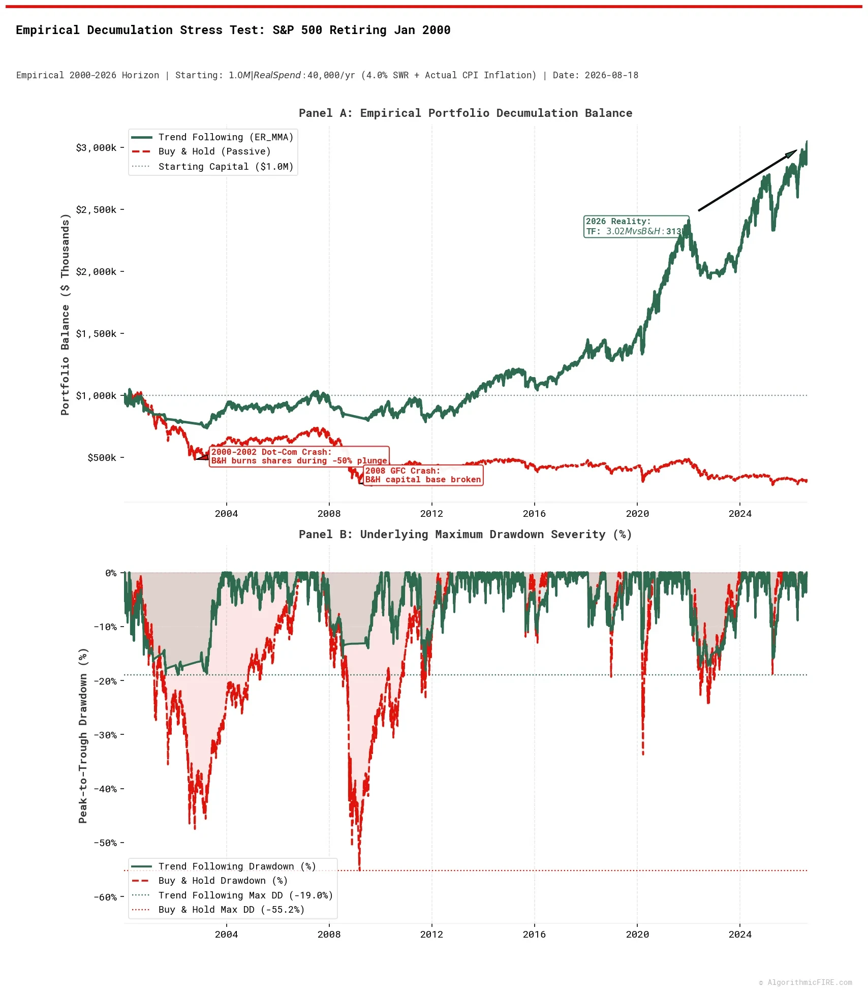
- Buy & Hold (Passive SPY):
- As stock prices plunged from 2000 to 2002, the retiree was forced to liquidate depressed shares at market lows to fund living expenses.
- By the time the 2008 crash hit, the capital base was irreversibly impaired. The portfolio dropped to a trough balance of $274,690 (-55.2% max drawdown) and ended August 2026 with just $313,442 remaining (a severe loss of real purchasing power after 26 years).
- Systematic Trend Following (ER_MMA):
- Moving average exit rules rotated exposure to cash and T-bills during the 2000–2002 bear market and the 2008 financial crisis.
- Living expenses were paid from sheltered cash and Treasury yield rather than selling battered equities.
- The lowest balance reached throughout the entire 26-year horizon was $733,453 (-19.0% max drawdown). By August 2026, the portfolio compounded to $3,024,883 (+$2,711,441 more wealth than passive Buy & Hold).
Case 2: Classic 60/40 Oct 2007 Retiree (60% Stocks / 40% Bonds)
A traditional balanced 60/40 portfolio is designed to protect retirees through bond diversification. But what happens during a severe credit crisis (2008) followed by a sharp inflation shock (2022, when stocks and bonds crashed simultaneously)?
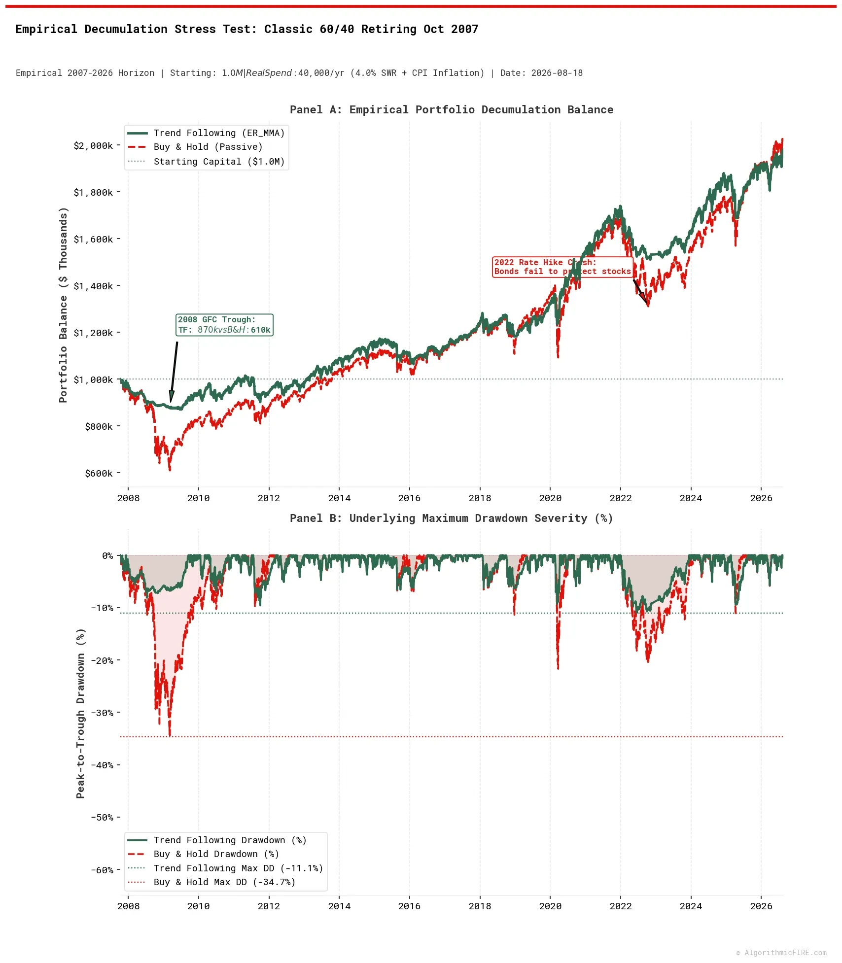
- Buy & Hold Classic 60/40:
- Plunged to a trough of $610,190 during the 2008 crash (-34.7% max drawdown).
- While it recovered during the 2010s bull market, the 2022 rate-hike shock caused severe double drawdowns in both equities and static bonds, ending August 2026 at $2,021,459.
- Systematic Trend Following (ER_MMA):
- Dynamic trend rules stepped out of equities in 2008 and rotated out of fixed income in 2022 as bond yields spiked.
- The portfolio's lowest trough balance was $870,186, bounding maximum drawdown to just -11.1% (a 68.1% drawdown reduction).
- It ended August 2026 at $1,971,150, delivering near-identical terminal capital while sparing the retiree from two severe multi-year drawdowns.
💡 Replacing Static Bonds with Trend Following
In my companion post, Can You Safely Retire on a 100% Stock Portfolio?, I showed that holding static fixed-income allocations imposes an expensive, permanent performance drag during economic expansions—and still fails during periods of high inflation.
Systematic trend following replaces the volatility-dampening role of bonds with dynamic risk management, allowing investors to compound on an equity growth base during bull markets while automatically stepping into cash during systemic downturns.
3. The Decumulation Break-Even Trap: Why Drawdowns Cause Irreversible Capital Impairment
To understand why peak drawdown depth dictates retirement survival, look at the mathematical relationship between drawdown depth and the return required to break even when taking living distributions.
During accumulation (0% withdrawals), the required rebound (R_{\text{accum}}) to restore capital follows the textbook recovery formula:
$$R_{\text{accum}} = \frac{D}{1 - D}$$
where (D) is the peak-to-trough drawdown depth expressed as a decimal ((0 < D < 1)). For example, a -20% drop ((D = 0.20)) requires a +25.0% rebound to break even, while a -50% drop ((D = 0.50)) requires a +100.0% rebound.
In decumulation, however, you must continue withdrawing money to pay living expenses while the portfolio is underwater.
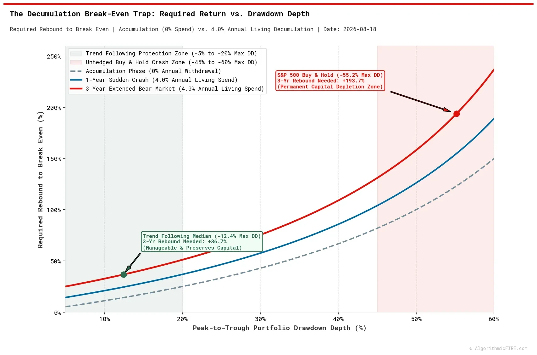
Key Takeaways from the Decumulation Break-Even Curves:
-
1-Year Sudden Crash (4.0% Living Spend):
- If a portfolio suffers a 1-year crash of depth (D) and pays a 4.0% annual distribution, the remaining balance after Year 1 is (B_1 = (1 - D) - 0.04 = 0.96 - D).
-
To restore the initial principal base of $1.00 and fund Year 2's $0.04 distribution (target balance (1.04)), the required rebound is: $$R_{1\text{-yr}} = \frac{1.04 - B_1}{B_1} = \frac{D + 0.08}{0.96 - D}$$
-
At a -20% drawdown ((D = 0.20)), the required rebound is +36.8%.
- At a -50% drawdown ((D = 0.50)), the required rebound jumps to +126.1%.
- At a -55% drawdown ((D = 0.55), matching the S&P 500 Dot-Com and 2008 crashes), the required rebound jumps to +153.7%.
-
3-Year Extended Bear Market (4.0% Living Spend):
- In extended bear markets (such as 2000–2002 or 2007–2009), withdrawals are deducted across multiple down years on a shrinking capital base.
- At a -20% peak drawdown, the 3-year required rebound is +51.1% (trough balance stays high at $688k per $1M).
- At a -50% peak drawdown, the 3-year required rebound spirals to +158.0% (trough balance drops to $403k).
- At a -55% peak drawdown, the required rebound spirals to +192.3% (trough balance drops to $356k).
-
The Exponential Destruction Zone:
- For an equity portfolio generating 7% to 10% annualized long-term returns, recovering from a +50% deficit takes a few years of normal compounding.
- Recovering from a +190% deficit while continuing to withdraw 4% each year is mathematically impossible without extraordinary luck. The portfolio enters a death spiral where living expenses consume an ever-increasing percentage of remaining assets.
- Trend following's mechanical exit rules keep maximum drawdowns in the green zone (-5% to -20%), preventing the portfolio from ever entering the exponential destruction zone.
4. Why I Prioritize Downside Protection in Portfolio Engineering
This mathematical reality explains why I structure my performance models and model portfolios around risk mitigation rather than raw compounding alone:
- Max Drawdown is the Primary Risk Factor: In my multi-period performance tables, I place Maximum Drawdown at the top. Cutting drawdowns from -55% to -12% is the primary engine of retirement longevity.
- Risk-Adjusted Efficiency (Sharpe & Sortino): When evaluating strategies, measuring return per unit of risk tells you far more about retirement survival than gross CAGR:
- Sharpe Ratio: Measures excess return per unit of total annualized volatility (both upside gains and downside drops). A higher Sharpe indicates cleaner, more consistent returns per unit of price fluctuation.
- Sortino Ratio: Isolates harmful downside volatility only. Unlike Sharpe, Sortino does not penalize upside volatility (sharp upward surges), focusing strictly on the negative return variance that threatens capital preservation.
- Cash as an Active Asset: When trend following models exit to cash or short-term Treasuries during extended market declines, that idle capital is not "wasted time." It preserves principal, earns risk-free yield, and prevents the devastating share-depletion that causes retirement failure.
5. Empirical Model Portfolio Drawdown Shield & Risk Efficiency Audit
I audited the empirical performance across all 10 curated model portfolios on the platform across their full live ETF histories (spanning 9.7 to 20.9 years, with an empirical median of 15.8 years).
I compared passive Buy & Hold directly against systematic trend following (Excess Return MMA / Advanced) over the exact same historical windows.
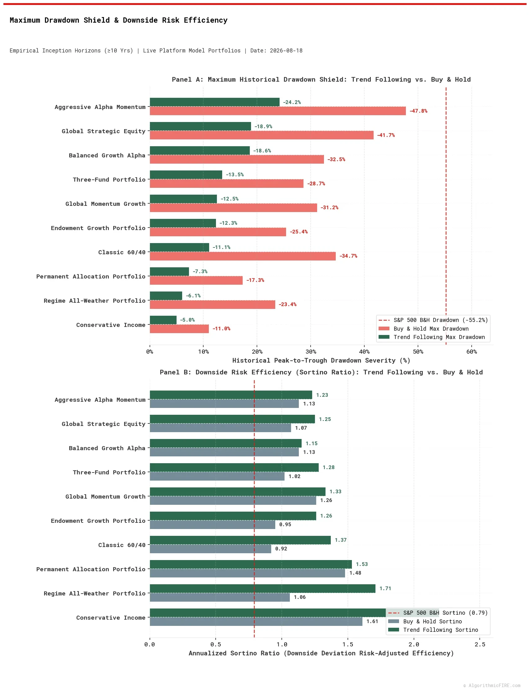
Empirical Model Portfolio Backtest Table (Common Horizons ≥10 Years)
| Model Portfolio / Strategy | Common Horizon | B&H CAGR | B&H Vol | B&H Max DD | B&H Sharpe | B&H Sortino | ER_MMA CAGR | ER_MMA Vol | ER_MMA Max DD | ER_MMA Sharpe | ER_MMA Sortino | Drawdown Shield |
|---|---|---|---|---|---|---|---|---|---|---|---|---|
| S&P 500 (SPY) (Benchmark) | 1993–2026 (33.5y) | 10.55% | 18.40% | -55.19% | 0.64 | 0.79 | — | — | — | — | — | — |
| Classic 60/40 (Advanced) | 2005–2026 (20.9y) | 8.41% | 11.68% | -34.70% | 0.75 | 0.92 | 7.91% | 7.17% | -11.06% | 1.10 | 1.37 | +23.64% (68.1% cut) |
| Conservative Income (Advanced) | 2009–2026 (17.3y) | 4.95% | 3.83% | -11.02% | 1.28 | 1.61 | 4.59% | 2.69% | -4.98% | 1.69 | 2.19 | +6.04% (54.8% cut) |
| Permanent Allocation Portfolio (Advanced) | 2009–2026 (17.2y) | 7.60% | 7.04% | -17.32% | 1.08 | 1.48 | 6.63% | 5.77% | -7.31% | 1.14 | 1.53 | +10.01% (57.8% cut) |
| Balanced Growth Alpha (Advanced) | 2009–2026 (17.0y) | 15.74% | 18.15% | -32.46% | 0.90 | 1.13 | 10.67% | 11.64% | -18.63% | 0.93 | 1.15 | +13.83% (42.6% cut) |
| Global Momentum Growth (Advanced) | 2009–2026 (17.0y) | 11.01% | 11.88% | -31.18% | 0.94 | 1.26 | 8.46% | 8.33% | -12.52% | 1.02 | 1.33 | +18.66% (59.8% cut) |
| Aggressive Alpha Momentum (Advanced) | 2012–2026 (14.5y) | 24.49% | 29.25% | -47.76% | 0.90 | 1.13 | 16.33% | 16.86% | -24.18% | 0.98 | 1.23 | +23.58% (49.4% cut) |
| Global Strategic Equity (Advanced) | 2012–2026 (14.5y) | 17.77% | 22.22% | -41.72% | 0.85 | 1.07 | 12.69% | 13.18% | -18.87% | 0.98 | 1.25 | +22.85% (54.8% cut) |
| Endowment Growth Portfolio (Advanced) | 2012–2026 (14.0y) | 8.36% | 11.22% | -25.41% | 0.77 | 0.95 | 6.94% | 7.12% | -12.33% | 0.98 | 1.26 | +13.08% (51.5% cut) |
| Three-Fund Portfolio (Advanced) | 2013–2026 (13.5y) | 10.75% | 13.41% | -28.67% | 0.83 | 1.02 | 9.56% | 9.31% | -13.50% | 1.03 | 1.28 | +15.17% (52.9% cut) |
| Regime All-Weather Portfolio (Advanced) | 2016–2026 (9.7y) | 6.71% | 8.82% | -23.37% | 0.78 | 1.06 | 7.09% | 5.37% | -6.06% | 1.31 | 1.71 | +17.31% (74.1% cut) |
| Trend Following Median (All 10) | 15.8y Median | 9.58% | 11.78% | -29.93% | 0.88 | 1.10 | 8.19% | 7.75% | -12.43% | 1.02 | 1.31 | +16.24% (54.8% cut) |
| Trend Following Mean (All 10) | 15.6y Mean | 11.58% | 13.75% | -29.36% | 0.91 | 1.16 | 9.09% | 8.74% | -12.94% | 1.12 | 1.43 | +16.42% (56.6% cut) |
Key Takeaways
- Universal Drawdown Shield:
- In 10 out of 10 model portfolios (100%), trend following cut maximum historical drawdown severity substantially.
- Across the entire suite, median peak drawdown was slashed from -29.93% down to -12.43%—a median +16.24% Drawdown Shield (54.8% reduction in peak loss).
- In high-beta strategies like Aggressive Alpha Momentum and Global Strategic Equity, trend following cut drawdowns by over 22% to 23%.
- Systematic Sortino Downside Efficiency Boost:
- In 10 out of 10 model portfolios (100%), trend following expanded the Sortino ratio.
- The median Sortino ratio rose from 1.10 to 1.31 (+0.21 improvement), and the median Sharpe ratio rose from 0.88 to 1.02.
- This proves that trend following does not simply cut risk by sacrificing return; it eliminates uncompensated downside volatility, making every unit of risk work harder for the retiree.
- Transparent Trade-off on Bull Market CAGR:
- In secular bull markets (such as 2009–2026), raw unhedged equity portfolios compound at high nominal rates because they experience no multi-year depressions. Moving partially to cash during shallow market pullbacks creates a modest tracking drag on CAGR.
- However, retirees do not fail because they earned 8.2% instead of 9.6%. Retirees fail because their portfolio loses -35% to -55% while they are forced to withdraw living expenses.
- Trend following trades a modest portion of peak bull-market compounding in exchange for structural protection against catastrophic sequence risk.
Decumulation Withdrawal Methodology & CPI Indexing
- Annual Inflation Step-Up: Empirical retirement decumulation simulations follow standard financial planning methodology. Starting with a 4.0% initial withdrawal ($40,000 on $1,000,000), dollar living distributions step up each January based on the cumulative trailing change in the headline Consumer Price Index for All Urban Consumers (FRED CPI-U /
CPIAUCNS). - Annual vs. Monthly Indexing: Stepping up spending annually (rather than monthly) reflects real-world retiree behavior (setting an annual household budget) and avoids the artificial compounding drag of high-frequency monthly inflation adjustments during volatile commodity spikes.
💡 Explore the Tools: You can model custom decumulation paths using the Interactive Calculators or inspect live trend-following allocations across the Model Portfolios.