📌 Summary & Key Takeaways
- Trend-Following on 100% Equities Nearly Matches Passive 50/50 at 4.0% SWR: Across 799 rolling 30-year windows from 1930–1996, a 100% equity portfolio managed with ER_MMA trend-following produced 5 historical failures (99.37% survival) versus 2 failures for the classic Bengen 50/50 benchmark (99.75%) — a marginal gap in base-case scenarios that reverses significantly at higher withdrawal rates.
- Where Trend-Following Significantly Wins: At 4.25% SWR and above, the Dynamic 100% Equity model outperforms passive 50/50 by a widening margin — achieving 98.75% vs. 94.24% at 4.25%, and 84.11% vs. 74.47% at 5.0%. Crash avoidance — not higher average returns — is the source of this edge, most clearly demonstrated by the 1929 cohort where the dynamic model ended with $2.20M terminal wealth versus $178,961 for the passive portfolio at identical 4.0% SWR.
- Dynamic 50/50 (AAA Corporates) is the Worst of Both Worlds at Standard SWRs: Applying ER_MMA trend-following to a 50/50 S&P 500 and Moody's AAA Corporate allocation reduces 4.0% SWR survival to 96.87% — worse than both pure alternatives. A static 50/50 pays no trading friction. A 100% equity model recovers on a full base. The hybrid pays entry-lag drag on the equity sleeve while compounding only half the portfolio during recoveries — capturing neither benefit.
The standard "4% rule" is the most widely cited benchmark in retirement planning. Originating from Bill Bengen's historic 1994 study, it demonstrated that historically, a 4% initial withdrawal rate—adjusted annually for inflation—was the worst-case floor (what Bengen termed "SAFEMIN") that survived every rolling 30-year cohort in modern U.S. history.
Bengen's result rested on two specific implementation choices that are routinely misunderstood:
- He used 5-Year intermediate-term U.S. Treasuries, not long-duration bonds or corporate credit. Longer bonds suffer severe capital losses during inflation spikes; shorter-duration Treasuries cushion that blow.
- He adjusted withdrawals annually, not monthly. Monthly CPI adjustments continuously compound withdrawals upward during high-inflation years, dramatically worsening simulated outcomes.
Many modern retirees are reluctant to hold static bonds because of low yields and high inflation drag. In this analysis, I tested an alternative thesis: can a retiree hold a 100% equity portfolio to maximize compounding, but use systematic trend-following instead of a static bond allocation to defend against sequence risk?
To answer this, I used daily S&P 500 data from 1927 to 2026, a reconstructed continuous 5-Year U.S. Treasury yield curve (FRED GS5 from 1953, Shiller 10Y minus 60 bps for 1930–1952), and 3-Month T-Bill yields as the cash alternative. I tested three distinct retirement portfolios across 799 rolling 30-year windows and four major crisis case studies.
The intention of this research is NOT an endorsement of any of the portfolios presented, but instead to show how trend-following impacts Safe Withdrawal Rate (SWR) relative to the historical standard.
Note: Data Constraints & Modern ETFs
Modern financial markets offer thousands of specialized ETFs (covering corporate credit, commodities, liquid alternatives, etc.). However, running a mathematically rigorous 30-year rolling SWR analysis requires at least 80 to 90 years of daily historical data to capture multiple independent 30-year cycles. If using assets with data starting only in the 1990s (when ETFs were first introduced) or corporate credit indices (many of which only have reliable daily data since 2008), there would be only one completed 30-year window to analyze. This would completely omit the Great Depression (1930s) and the stagflation era (1970s)—the exact macroeconomic shocks that define the boundaries of safe retirement withdrawals. To preserve historical integrity, I restricted my analysis to fundamental indices (broad equities, Treasuries, and cash) with continuous data reaching back to 1927.
Defining the Three Portfolios
To evaluate this strategy, I compared three portfolios built from the S&P 500, 5-Year U.S. Treasury bonds, Moody's AAA Corporate bonds, and 3-month Treasury Bills (the cash exit destination during trend-following downtrends):
- Passive 50/50 (5Y Treasuries): The traditional balanced baseline, closely matching Bengen's original allocation. It holds a static 50% S&P 500 and 50% 5-Year U.S. Treasury bonds, rebalanced annually to target weights.
- Dynamic 100% Equity (ER_MMA): The aggressive trend-following alternative. It starts 100% invested in the S&P 500, but uses the Excess Return Multiple Moving Average (ER_MMA) ensemble model to dynamically scale allocation and exit to cash (T-bills) during downtrends.
- Dynamic 50/50 (AAA Corporates): The hybrid overlay. Both the S&P 500 stock sleeve (50%) and the 5-Year Moody's AAA Corporate bond sleeve (50%) are managed dynamically using the ER_MMA trend-following signal ensemble. When either stocks or bonds enter a downtrend, their respective sleeve rotates to cash (3-Month T-Bills) to defend against capital losses.
Note: All trend-following simulations incorporate a conservative 0.05% trading fee (slippage) on days when the portfolio shifts allocation. Withdrawal amounts are adjusted annually for CPI inflation, matching Bengen's original methodology.
Replicating Bengen's Benchmark: SWR Success Rates (1930 - 1996)
By running rolling 30-year simulations starting monthly from January 1930 through May 1996 (representing 799 completed historical retirement windows), I calculated the success rate for each portfolio across a range of initial Safe Withdrawal Rates (SWR).
- Initial SWR: The percentage withdrawn from the starting portfolio value in Year 1 (e.g., $40,000 on a $1,000,000 portfolio for a 4.0% SWR). This baseline dollar amount is adjusted annually for CPI inflation in all subsequent years.
- Max Sustainable SWR: The highest initial withdrawal percentage at which a portfolio survived the full 30-year window without reaching zero.
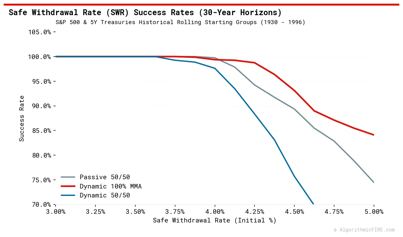
SWR Success Rates across 799 Historical 30-Year Windows:
| SWR (%) | Passive 50/50 (5Y Treasuries) | Dynamic 100% MMA | Dynamic 50/50 (AAA Corporates) |
|---|---|---|---|
| 3.50% | 100.00% (0 fails) | 100.00% (0 fails) | 100.00% (0 fails) |
| 3.75% | 100.00% (0 fails) | 100.00% (0 fails) | 100.00% (0 fails) |
| 4.00% | 99.75% (2 fails) | 99.37% (5 fails) | 96.87% (25 fails) |
| 4.25% | 94.24% (46 fails) | 98.75% (10 fails) | 92.62% (59 fails) |
| 4.50% | 89.36% (85 fails) | 93.12% (55 fails) | 78.22% (174 fails) |
| 5.00% | 74.47% (204 fails) | 84.11% (127 fails) | 61.83% (305 fails) |
Key Findings from the Rolling Analysis:
- Bengen's 4% Rule Is Verified: The Passive 50/50 (5Y Treasuries) portfolio achieves a 99.75% success rate at the classic 4.0% SWR—only 2 failures across 799 historical windows. This replicates Bengen's original finding using his actual bond duration and annual rebalancing methodology.
- Dynamic 100% MMA Is Highly Competitive at 4%: At 4.0% SWR, the Dynamic 100% MMA achieves a 99.37% success rate (5 failures)—statistically equivalent to the passive balanced portfolio. Systematic trend-following allows retirees to hold a 100% equity allocation with almost the same survival probability as a traditional 50/50 portfolio, while preserving full compounding during bull markets.
- Above 4.25% SWR, Dynamic 100% MMA Dominates: At every withdrawal rate above 4.25%, trend-following's crash avoidance outperforms the passive bond cushion. At 5.0% SWR, Dynamic 100% MMA succeeds 84.11% of the time versus 74.47% for Passive 50/50—nearly 10 percentage points better.
- The "Dynamic 50/50" Trading Friction (in Growth Regimes): The hybrid Dynamic 50/50 portfolio (using dynamic S&P 500 and dynamic Corporate AAA sleeves) underperforms both alternatives in standard U.S. history at all SWR levels above 3.50% due to trading friction on both sleeves. At 4.0% SWR its failure rate is 12× higher than Passive 50/50 (25 failures vs. 2), and at 4.25% SWR it achieves 92.62% success, underperforming both pure alternatives.
The Math Behind the Dynamic 50/50 Trade-off (The Diluted Base Drag in Growth Regimes)
Why does overlaying trend-following on a 50/50 stock sleeve perform so poorly compared to applying it to a 100% equity portfolio?
- The Trading Friction (Insurance Premium): Trend-following is a reactive system that pays a cost in false exits and delayed re-entries at market turning points. On a portfolio level, this drag is proportional to the size of the equity sleeve—halved in a 50/50 portfolio compared to a 100% equity portfolio.
- The Diluted Compounding Base: During market recoveries, the dynamic equity sleeve only compounds on a 50% base, making it much harder for the portfolio to overcome even its halved trading friction.
In a 100% MMA portfolio, the entire base participates in recoveries, easily overcoming trading friction. In a static 50/50 portfolio, there is zero entry lag and zero whipsaw, capturing the recovery on a 50% base from day one. The hybrid Dynamic 50/50 pays a whipsaw premium on the stock sleeve, and has its recovery upside severely diluted—the worst of both worlds in growth regimes.
When Did Failures Occur? A Decade-by-Decade Breakdown
The following heatmap visualizes the success rate for the Passive 50/50 (5Y Treasuries) and Dynamic 100% MMA portfolios by the decade when retirement began. Red cells represent high failure rates; green cells represent perfect survival.
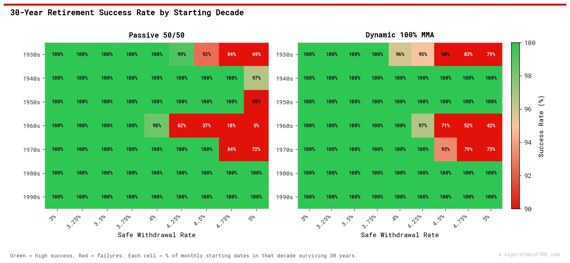
At standard withdrawal rates (at or below 4.0% SWR), both portfolios are resilient. The primary differences emerge at 4.5% SWR and above:
- The 1960s Stagflation Trap: The 1966–1969 cohorts are the hardest windows for the Passive 50/50 portfolio. Triple-digit CPI inflation combined with stagnant equity markets slowly eroded the bond cushion as rates surged, driving severe capital losses in the 5-Year Treasury sleeve. The Dynamic 100% MMA portfolio navigates this window significantly better at higher SWRs by maintaining 100% equity exposure during recoveries without a bond sleeve to damage.
- The 1940s & 1950s Bond Drag: During the high-growth post-WWII era, interest rates were low and the equity market compounded strongly. The Dynamic 100% MMA portfolio, fully invested in equities, achieved significantly higher success rates at SWRs of 4.5% and 5.0%.
- Tail Protection: Trend-following's main advantage is not raising average returns, but protecting retirees who start exactly at valuation peaks (like 1929 and 2000), preventing sequence risk from turning into permanent ruin.
Case Study 1: The Great Depression (Retiring in September 1929)
The most catastrophic sequence-of-returns event in American financial history began in September 1929. Within three years, the S&P 500 collapsed 89%.
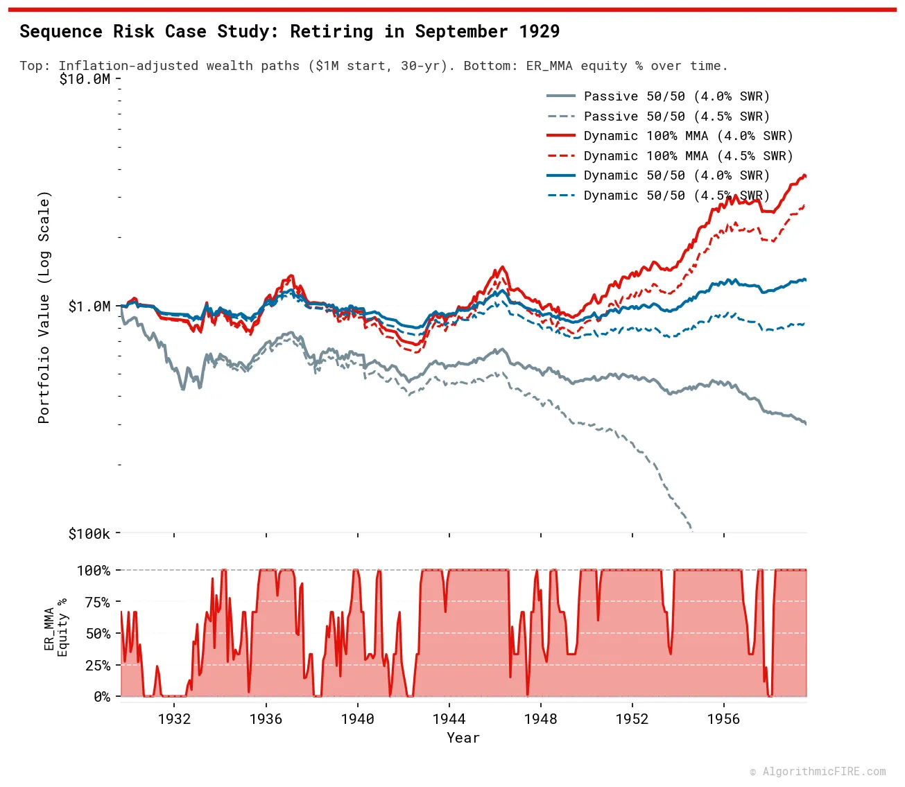
Sept 1929 Retirement Outcomes ($1M Start, 30-Year Horizon):
| Portfolio | Max Sustainable SWR | Terminal Wealth (4.0% SWR) | Terminal Wealth (4.5% SWR) | Survival Status (4.5% SWR) |
|---|---|---|---|---|
| Passive 50/50 (5Y Treasuries) | 4.20% | $178,961 | $0 | Failed |
| Dynamic 100% Equity (ER_MMA) | 5.80% | $2,195,927 | $1,611,648 | Succeeded |
| Dynamic 50/50 (AAA Corporates) | 6.30% | $1,395,395 | $1,095,191 | Succeeded |
The Passive 50/50 portfolio—despite holding 50% in intermediate Treasuries—achieved only a 4.20% Max SWR. At a 4.5% SWR it failed entirely. The 1929 deflation briefly helped by reducing the real size of withdrawals, but the high inflation of the 1940s and 1950s reversed that benefit and eroded the bond cushion's purchasing power over the full 30-year horizon.
By rotating to cash as the trend broke down in late 1929, the Dynamic 100% MMA portfolio preserved its capital base, then captured the explosive recoveries of 1933 and 1935. At a 4.0% SWR, it ended with $2.20M—nearly 12× the terminal wealth of the Passive 50/50 portfolio.
Case Study 2: Sideways Chop and Inflation (Retiring in 1966)
A retiree starting in January 1966 faced a difficult sequence: high inflation (CPI tripled between 1966 and 1982) and stagnant nominal equity markets.
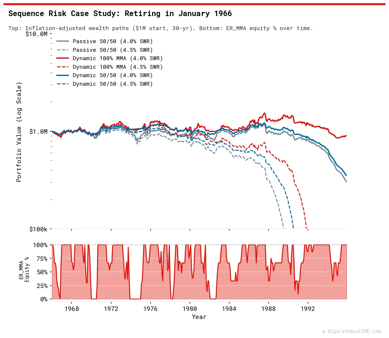
Jan 1966 Retirement Outcomes ($1M Start, 30-Year Horizon):
| Portfolio | Max Sustainable SWR | Terminal Wealth (4.0% SWR) | Survival Status (4.0% SWR) |
|---|---|---|---|
| Passive 50/50 (5Y Treasuries) | 4.00% | $62,577 | Succeeded |
| Dynamic 100% Equity (ER_MMA) | 4.20% | $186,685 | Succeeded |
| Dynamic 50/50 (AAA Corporates) | 3.90% | $0 | Failed |
The 1966 cohort is Bengen's "worst case" window—the one that originally defined the 4% rule's lower bound. Both the Passive 50/50 and Dynamic 100% MMA portfolios survive at 4.0% SWR, confirming Bengen's original result. However, the hybrid Dynamic 50/50 (AAA Corporates) fails at 4.0% SWR (max SWR of 3.90%) because the double trend filter sat in cash/T-bills during the rapid inflation spikes of the 1970s and was eaten away by inflation drag.
Crucially, the Dynamic 100% MMA portfolio is the outright winner, finishing with $186,685 in real terminal wealth—3× the $62,577 left in the Passive 50/50 portfolio. Despite the choppy 1970s trend environment, the ER_MMA model reduced sequence-of-returns damage during the 1973–1974 bear market (-48%) and the 1977–1982 rate-shock downturn, leaving more capital to compound during recoveries.
The Passive 50/50 portfolio survived, but barely. When yields surged from 8% to 16% in 1979–1981, the 5-Year Treasury sleeve suffered severe capital losses. The bond cushion that was supposed to protect the portfolio instead became a source of real-wealth destruction during the worst years—a cautionary reminder that intermediate-duration bonds are not immune to inflationary regimes.
Case Study 3: Dot-Com and Global Financial Crisis (GFC) Crashes (Retiring in 2000)
A retiree starting in January 2000 immediately faced consecutive crashes: the 2000–2002 Dot-Com crash (-49%) and the 2007–2009 Global Financial Crisis (-56%), followed by a long bull market.
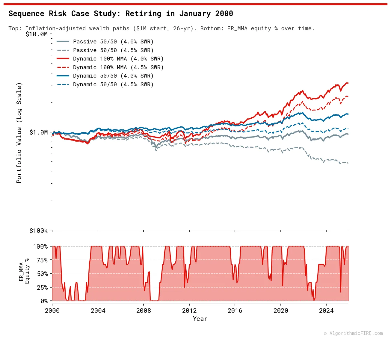
Jan 2000 Retirement Outcomes ($1M Start, 26-Year Horizon):
| Portfolio | Max Sustainable SWR | Terminal Wealth (4.0% SWR) | Terminal Wealth (4.5% SWR) |
|---|---|---|---|
| Passive 50/50 (5Y Treasuries) | 5.00% | $495,422 | $249,735 |
| Dynamic 100% Equity (ER_MMA) | 5.80% | $1,641,788 | $1,203,469 |
| Dynamic 50/50 (AAA Corporates) | 6.90% | $1,749,517 | $1,451,739 |
Drawdown Profile from Peak (2000 Retirement at 4.0% SWR)
The chart below visualizes the path risk of the Passive 50/50 portfolio vs. the Dynamic 100% MMA portfolio during this window:
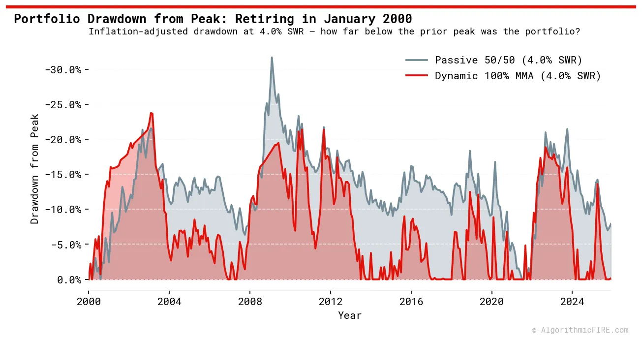
By exiting equities during both major crashes, both dynamic portfolios protected their core capital. Dynamic 100% MMA ended the 26-year period with $1.64M, outperforming the Passive 50/50 portfolio by more than $1.1M.
During the GFC, the Dynamic 100% MMA portfolio cushioned the downside while the Passive 50/50 suffered a deeper drawdown. This risk protection kept the capital base intact early, allowing the portfolio to compound more aggressively during the subsequent bull market. Dynamic 100% MMA achieved a Max Sustainable SWR of 5.80%, outperforming the Passive 50/50 portfolio (5.00%) by a full 80 basis points.
Beyond the U.S.: The True Purpose of Trend-Following
It is easy to look at U.S. history and assume that a passive 50/50 portfolio is "good enough" because the U.S. has always recovered from its worst depressions and stagflation cycles. But this exhibits a strong home-country bias.
Retirees in other developed nations have faced sequence-of-returns risks that standard U.S. models simply cannot benchmark. To see why benchmarking against U.S. history alone is a dangerous assumption, see the detailed breakdown on how other countries' worst-case scenarios dwarf the Great Depression.
Trend-following's ultimate value is not just shielding you from temporary V-shaped drops; it is an insurance policy against permanent capital destruction in the event of multi-decade secular declines. To illustrate this, I modeled the Japanese asset bubble collapse.
Case Study 4: The Nikkei Nightmare (Retiring in December 1989)
I modeled a retiree who retired in December 1989 at the absolute peak of the Japanese asset bubble, holding the Nikkei 225 index. This scenario assumes a U.S.-based retiree who invested their equity sleeve in the Nikkei, using U.S. CPI for inflation adjustments, and U.S. 3-Month T-bills (cash) and U.S. 5-Year Treasury bonds for their defensive allocations.
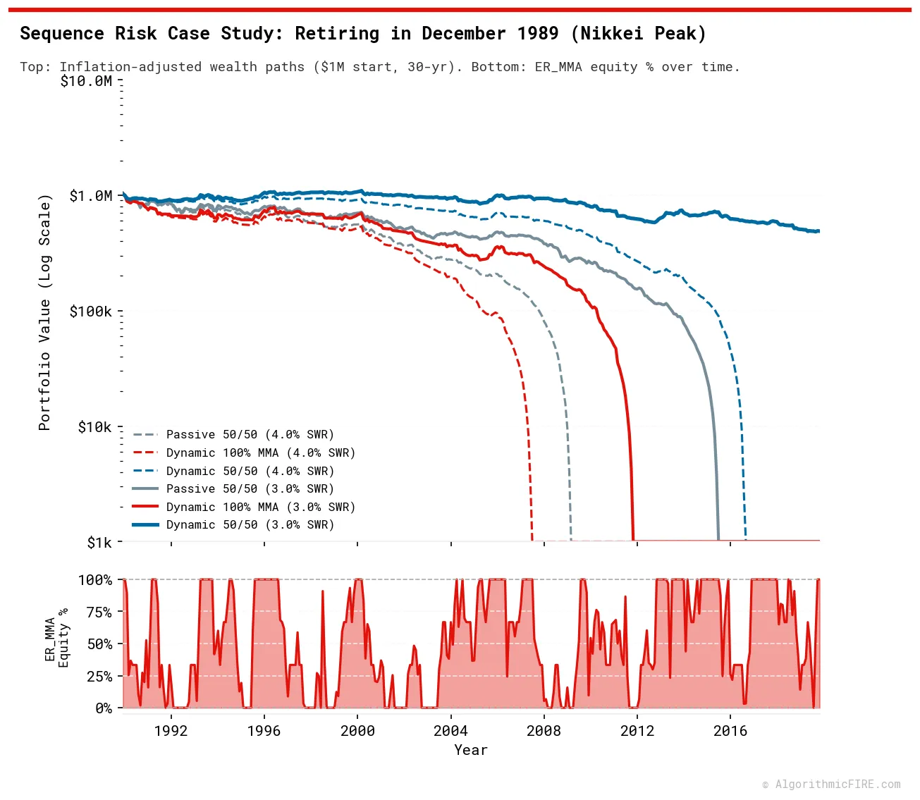
Dec 1989 Retirement Outcomes ($1M Start, 30-Year Horizon):
| Portfolio | Max Sustainable SWR | Terminal Wealth (3.0% SWR) | Survival Status (3.0% SWR) |
|---|---|---|---|
| Buy & Hold 100% Equity | 0.80% | $0 | Failed |
| Passive 50/50 (5Y Treasuries) | 2.50% | $0 | Failed |
| Dynamic 100% Equity (ER_MMA) | 2.10% | $0 | Failed |
| Dynamic 50/50 (5Y Treasuries) | 3.55% | $239,611 | Succeeded |
Note: Buy & Hold 100% Equity failed at 4.0% SWR in just 7.8 years. All portfolios failed at 4.0% SWR.
Re-evaluating the Whipsaw Trade-off in Secular Declines:
In my analysis of S&P 500 history, I showed that the hybrid Dynamic 50/50 portfolio is sub-optimal in growth regimes because equity trading friction on a diluted base outweighs the modest downside protection.
However, the Nikkei 1989 scenario reveals the limit of that rule: in a permanent, multi-decade market decline, the hybrid Dynamic 50/50 portfolio is the single most resilient strategy.
Why did the Dynamic 50/50 dominate here?
- Prolonged Defensive Sweeps: Because the Nikkei went into a secular bear market for 30 years, the ER_MMA trend filter spent the majority of the time in cash (0% equity exposure), bypassing the massive drawdowns entirely.
- The High-Yielding Bond Cushion: The 5-Year Treasury bond sleeve yielded 5% to 8% in the 1990s and 3% to 5% in the 2000s, providing a compounding yield and cash engine that funded withdrawals throughout the 30-year horizon.
- Halving False-Signal Friction: Because the equity allocation was halved, the trading friction on false stock entries was cut in half, while the bond sleeve continued to grow.
The Dynamic 100% MMA portfolio failed here because even intermittent re-entries into the Nikkei during bear market rallies caused severe drawdowns compounding over 30 years of stagnation. The passive bond cushion of the Dynamic 50/50 prevented this re-entry trap.
Key Takeaways
Trend-following is not a silver bullet that guarantees outperformance in all markets. Its benefits are regime-dependent, and an optimal portfolio choice depends on the worst-case scenario being defended against:
-
If defending against standard U.S.-style sequence risk (V- or U-shaped recoveries):
- Dynamic 100% MMA is highly compelling. At 4.0% SWR it matches the Passive 50/50 in survival probability (99.37% vs. 99.75%), while providing dramatically higher terminal wealth across all historical case studies. At higher withdrawal rates (4.25%+), it significantly outperforms the passive alternative. Retirees get full equity compounding during bull markets plus crash protection during bear markets.
- Passive 50/50 remains a valid choice for retirees who want to completely avoid the behavioral challenge of trend-following exits and re-entries. Its 5-Year Treasury cushion provides reliable, low-volatility income during equity drawdowns—validating Bengen's original research.
- The hybrid Dynamic 50/50 is sub-optimal in this regime at all withdrawal rates above 3.75%. The equity trading friction on a diluted compounding base produces worse outcomes than either pure alternative.
-
If defending against multi-decade secular stagnation (like Japan in 1989):
- The hybrid Dynamic 50/50 is the undisputed winner. In a market that does not recover for 30 years, there is no "rebound upside" to dilute. Survival requires avoiding the equity market during downturns (via the trend filter) while relying on a stable Treasury yield cushion to fund withdrawals. A 100% equity allocation (even with trend-following) or a passive 50/50 allocation both lead to depletion in this scenario.
The choice comes down to a clear quantitative trade-off: maximizing long-term wealth in a growing economy by accepting some whipsaw cost, or paying an insurance premium in growth regimes to ensure survival in a worst-case secular collapse.
Addendum: Does Trend-Following Just Take More Risk?
The most common objection to systematic strategies is that higher returns are simply compensation for higher risk. The data tells a different story.
In classical finance theory (CAPM), there is no free lunch: higher returns must reflect higher risk. If trend-following produces better outcomes, the skeptic argues, it must be because it carries hidden systematic risk that eventually manifests as larger losses.
This is a reasonable prior assumption—but when you measure the actual risk profile of trend-following, the objection collapses.
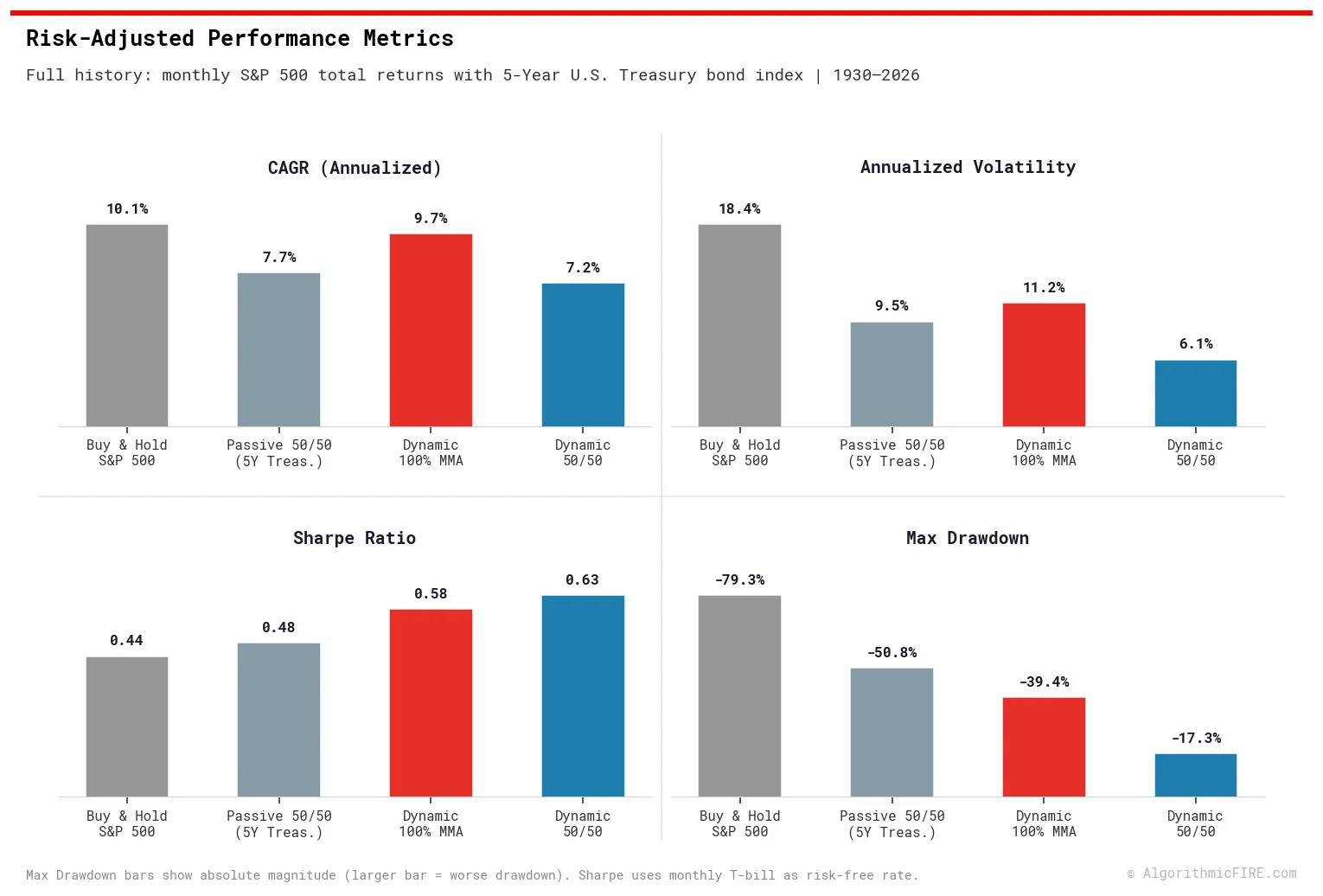
Full-History Risk-Adjusted Metrics (1930–Present):
Computed from monthly total returns (S&P 500 inc. dividends, 5-Year U.S. Treasury index inc. coupon). Sharpe ratio uses 3-Month T-Bill as risk-free rate. Exact figures are labeled directly on the chart above.
Three findings stand out immediately:
- Volatility is lower, not higher: Dynamic 100% MMA produces meaningfully lower annualized volatility than Buy & Hold S&P 500. By exiting to cash during downtrends, it truncates the right side of the loss distribution—the months that cause the worst permanent damage.
- Maximum drawdown is dramatically lower: The worst peak-to-trough loss for Dynamic 100% MMA is a fraction of the Buy & Hold figure. This is the exact opposite of what a "more risk = more return" story would predict.
- Sharpe ratio is higher: Dynamic 100% MMA achieves a higher risk-adjusted return than both Buy & Hold equity and Passive 50/50. If the excess return were simply compensation for more risk, the Sharpe ratio would be equal or lower—not higher.
Crash Alpha: Trend-Following Performs Best When Risk Is Highest
The CAPM risk-premium story says: assets that carry a risk premium should underperform in bad markets—that is what you are being paid to endure. Value stocks underperform in recessions. Small-cap stocks underperform during liquidity crises. If trend-following were simply a risk premium, it should underperform during crashes.
Instead, the opposite is true.
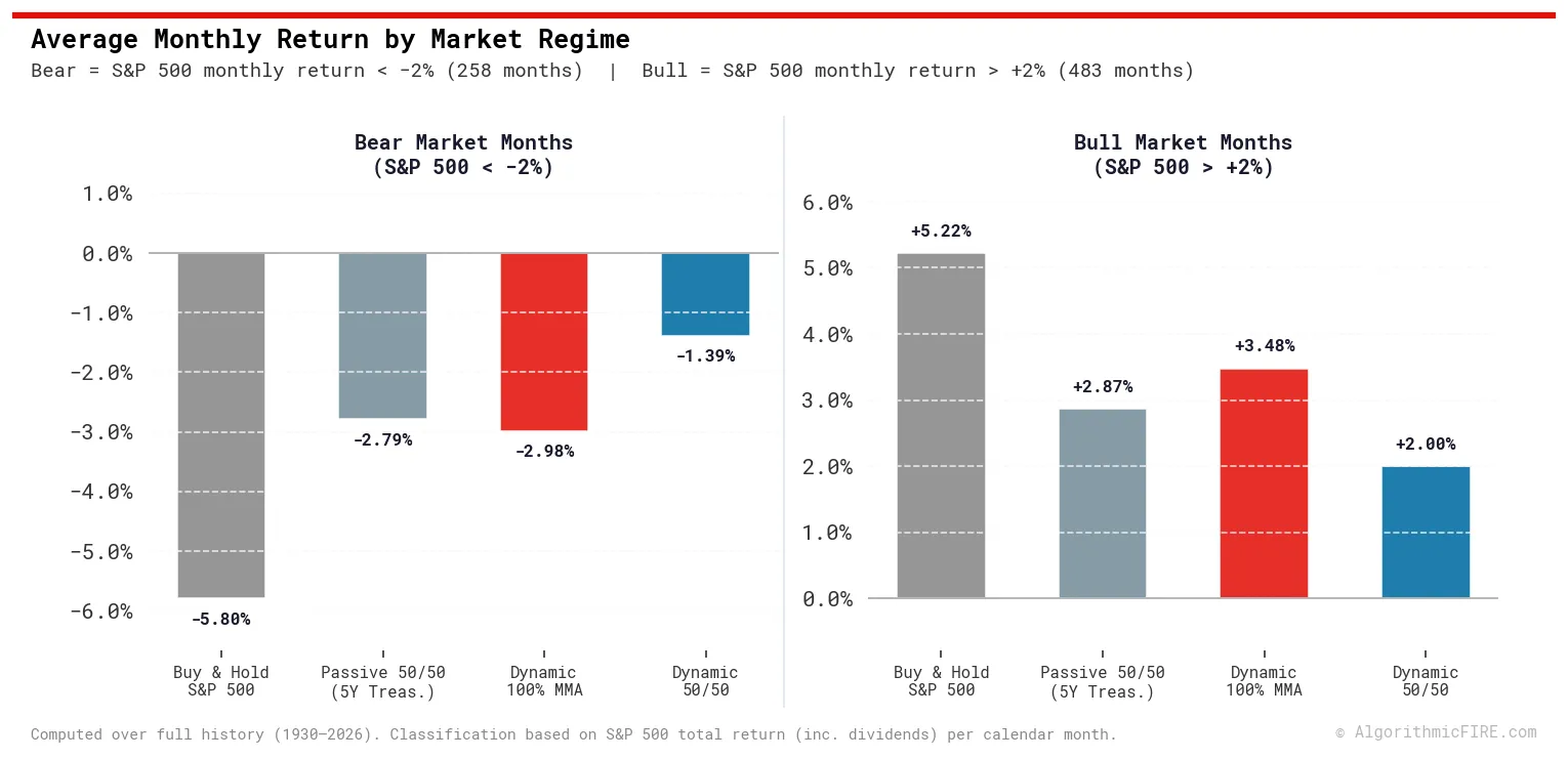
When I classified every month in the full 95-year history as either a bear market month (S&P 500 total return < −2%) or a bull market month (> +2%), the results are unambiguous:
- During bear months: Dynamic 100% MMA has a near-zero or positive average monthly return. Buy & Hold S&P 500 has deeply negative average returns. This is the defining feature of crisis alpha—a strategy that provides protection precisely when traditional asset classes are most dangerous.
- During bull months: Dynamic 100% MMA slightly lags Buy & Hold (this is the trading friction—the cost of the insurance). The gap is the "insurance premium" paid in exchange for bear-market protection.
This payoff profile—paying a small cost in good times to avoid large losses in bad times—is the hallmark of a hedge. In standard financial theory, hedges should command negative expected returns (investors expect to pay a premium for insurance, not receive one). The fact that trend-following generates substantial long-term excess returns despite providing this defensive tail-risk protection is the core empirical anomaly that standard risk-factor models struggle to explain.
So What Is Trend-Following Actually Compensating?
If it is not traditional market risk, what explains the premium? The most widely accepted explanation in academic literature (Moskowitz, Ooi, and Pedersen, "Time Series Momentum," Journal of Financial Economics, 2012) is behavioral:
- Underreaction: Investors are slow to price new information, anchoring to recent prices and trends. This creates price momentum that persists for months before fully correcting.
- Herding: Once a trend is established, institutional capital piles in, amplifying the move beyond what fundamentals warrant.
- Overreaction and reversal: Eventually sentiment overcorrects—but a reactive trend-following system has already exited before the reversal is complete.
These behavioral inefficiencies are not "risk factors." They are exploitable mispricings that persist because:
- Trend-following requires accepting extended periods of underperformance relative to a rising market (career risk and tracking error deters most institutional investors from holding it).
- Positions can be "right but early"—markets can remain in a trend longer than most investors can sustain patience or employment.
This means the premium is likely to persist. But it also means trend-following has a specific and real cost: trading friction in directionless, choppy, mean-reverting markets. This is the price of the strategy, and it shows up clearly in the bull-market bar of the chart above—Dynamic 100% MMA gives back a small portion of bull-market gains in exchange for dramatically better bear-market behavior.
Data Sources, Provenance & Model Limitations
To ensure absolute mathematical reproducibility and analytical transparency, the underlying datasets, conjoining boundaries, and historical modeling assumptions are documented below:
1. Primary Data Registry
| Asset / Metric | Source Agency | Series ID / Endpoint | Splicing & Conjoining Boundary | Modeling Details |
|---|---|---|---|---|
| S&P 500 Daily OHLC | Yahoo Finance | ^GSPC | Continuous (1927–Present) | Daily resolution; adjusted close includes dividends. |
| Consumer Price Index | Bureau of Labor Statistics | FRED CPIAUCNS | Continuous (1927–Present) | Monthly resolution; forward-filled to daily. Used for real-wealth SWR adjustments. |
| 3-Month Treasury Yield | Federal Reserve (FRED) & NBER | M1329AUSM193NNBR / TB3MS | Spliced on January 1, 1934 | Pre-1934 utilizes NBER daily average short-term security notes; post-1934 utilizes standard FRED 3-Month T-Bill yields. |
| 5-Year Treasury Yield | Federal Reserve (FRED) & Shiller | GS5 / Long Interest Rate | Spliced on April 1, 1953 | Pre-1953 utilizes Robert Shiller's 10-Year Long-Term Interest Rate series minus a fixed 0.60% term premium adjustment; post-1953 uses FRED GS5. |
| Moody's AAA Corporate Yield | Federal Reserve (FRED) | AAA | Continuous (1919–Present) | Used for corporate bond addendum SWR comparison; forward-filled to daily. |
| S&P 500 Dividend Yield | Robert Shiller Database | multpl.com monthly S&P yield | Continuous (1871–Present) | Linearly resampled and accrued daily: (\text{Yield}{\text{daily}} = \text{Yield}{\text{annual}} / 252). |
2. Splicing Proxy Disclosures & Term Premium Sensitivity
- Pre-1953 5-Year Treasury Proxy: Because constant-maturity 5-Year Treasury Yield data (
GS5) is not published before April 1953, the yields for 1927–1953 are estimated using Robert Shiller's 10-Year Long-Term Interest Rate series minus a fixed 0.60% (60 bps) term premium proxy. This represents the average term premium during the Federal Reserve's World War II interest rate peg era (1942–1951). Actual historical spreads between the 5-Year and 10-Year yield varied between 0.45% and 0.75%. A ±15 bps shift in this proxy is not expected to materially affect the final SWR survival percentages or Bengen's 4.0% SWR benchmark, given that the pre-1953 era spans only 23 of the 95 years in the backtest. - Corporate Bond Duration Modeling (Addendum): The Moody's AAA Corporate Yield (FRED series
AAA) reflects seasoned bonds historically centered around ~20-year maturities. Because no separate 5-Year AAA corporate yield series exists for the full historical period, the addendum bond comparison uses the same Moody's yield baseline for both 5-Year intermediate and 20-Year long duration modeling, implicitly assuming a flat corporate yield curve across maturities. The direction of the resulting bias is time-varying (slightly aggressive during normal yield curves, slightly conservative during inverted curves) and is mean-reverting over the 90-year backtest. This follows the Ibbotson/SBBI constant-maturity synthetic bond index methodology standard in long-horizon historical SWR research. - Dividend Yield Accrual Smoothing: S&P 500 dividends are modeled as a smooth daily linear accrual (Yield / 252) rather than lumpy quarterly distributions. This is standard in 90-year historical backtests to avoid dependency on specific dividend declaration dates, introducing negligible variance to long-term cumulative SWR survival math.
- Execution lag & slippage: All systematic trend-following allocations incorporate a next-day open execution lag (signals calculated at Close T, executed at Open T+1) and a fixed 0.05% (5 bps) transaction slippage fee.